Introduction

The advent of polymer technology are needed. Polymers are light weight, low cost and require low power consumption. The structure of the polymers are studied. There are progress on the fabrication methods of polymers. The elements in the polymer are studied using energy dispersive spectroscopy [1]. Basic measurements of the polymer are the weight and percentage of the elements. Recent studies are ongoing on polymers towards imaging to characterize the structure. The nanoparticle preparation provides the size of the particle using the scanning electron microscopy [2-4]. Surface roughness are studied to understand the tribology aspects of the polymers and materials [5-7]. The applications are many that include printing, energy [8-11] and battery [12,13]. The change in the structure during the fabrication are yet to be explored. Surface profilometer provides the surface geometry of the said polymer [14,15].

The common elements in the polymer are organic, metals and alloys. The chemical elements are carbon, oxygen and hydrogen. The metals include sodium, lithium, potassium, aluminum, magnesium, copper and molybdenum [16]. For instance, polystyrene are produced from carbon, hydrogen and oxygen. Researchers have studied polystyrene from the ethylene and benzene hybridization fabrication methods [17]. Polystyrene are thermoplastics. They are opaque, durable, insulators and their dye monomers are easy to obtain by powder based manufacturing. They are used in CDs, toys, brush, packages, displays and insulators. Vibrational sum-frequency generation spectroscopy probes the molecules using force. They give the element composition in polystyrene. Numerical simulations on polymers to understand the molecules arrangement are available [18]. Polyethylene oxide are plastics that are used in batteries [19]. Their structure are different from polystyrene with the similar chemical elements that include the carbon, oxygen and hydrogen. The preparation of the polyethylene oxide using ethylene glycol, dye provides transparent and translucent surfaces. The knowledge of metal-polymer matrix on current are studied [20]. The nanoparticles in operando visualization are towards the measurement of the power. In the recent years polyethylene oxide with lithium are studied [21-24].  Polyvinyl chloride pipes are heavy use in pipe flow and agriculture irrigation.  The elements in polyvinyl chloride are typical carbon, oxygen, hydrogen and chlorine. The fabrication of polyvinyl chloride from chemical vapor deposition are known [25,26]. The standard surface roughness parameters in polymers are studied using surface profilometer [27-32]. The cloth based polymers are investigated to understand the elements and surface roughness parameters [33-36].

In this paper, we study the five polymers that include polystyrene, transparent polyethylene oxide, translucent polyethylene oxide, polyvinyl chloride and textile cloth. We investigate the standard surface roughness parameters of our polymers for the first time. The surface roughness of the polystyrene with its high sensitivity to measure the material film are the novelty of the work. The surface roughness are characterized on the front and back side of the polystyrene. On the font side the surface roughness of polystyrene is 3.14 µm with the sensitivity of 0.01 μm. These findings are available as coating surface using polystyrene on quartz [37]. The thickness mentioned from measurements of coated polystyrene are 6 μm that gives the new perspective on substrate polymer with quartz in measurements to alloys. We perform scanning electron microscopy on the polymers. We study the chemical elements and their composition on our polymers one by one using energy dispersive spectroscopy. The standard surface roughness parameters on the textile cloth are studied. We investigate the surface roughness on the non-print and print regions in the cloth.

The rest of the paper is outlined as follows. Section 2 discusses the materials and methods. A detailed discussion on the surface roughness of polymers are given in Section 3. Finally, conclusions are presented in Section 4.

Material and Methods

The scanning electron microscopy equipment are from IITM facility. The surface profilometer are available in IITM facility. We purchase the four polymers that include polystyrene, transparent polyethylene oxide, translucent polyethylene oxide and polyvinyl chloride from Lakshmi electrical and hardwares, India. The Computer Aided Design (CAD) drawing are made using freeform app. The drawings are provided to Sj Woven Labels, India. The textile cloth are purchased from Sj Woven Labels, India. The computer aided design drawings are printed on the textile using woven label machine available in Sj Woven Labels, India. Table 1 shows the specification details and measurement conditions of the surface profilometer.

Results and Discussion

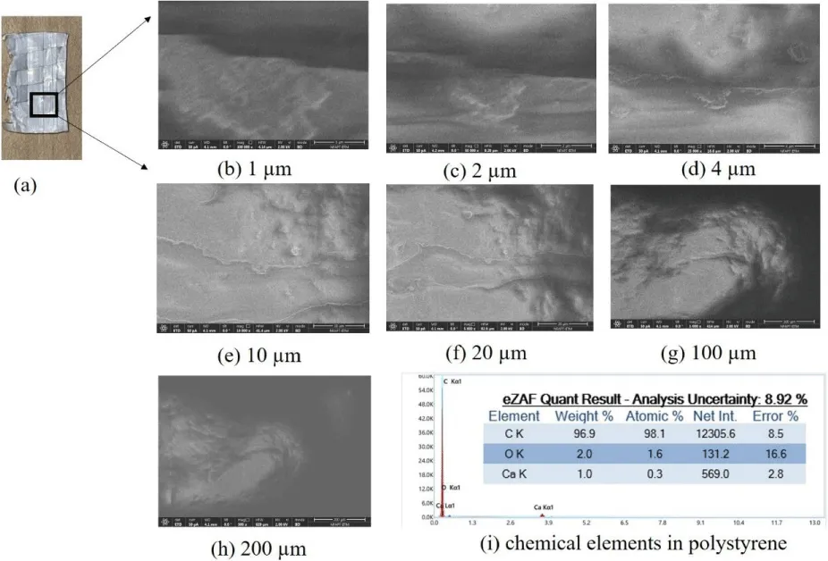
Figure 1 (a) shows the actual polystyrene. Figure 1 (b) shows 1 µm (c) 2 µm (d) 4 µm (e) 10 µm (f) 20 µm (g) 100 µm and (h) 200 µm imaging resolution. The scanning electron microscopy are used to image the polystyrene. Figure 1 (i) shows the materials present in the polystyrene. The elements are carbon, oxygen and calcium. The composition of carbon is 96.9 %, oxygen 2 % and calcium 1 %, respectively. We understand that the polystyrenes are organic clean polymers that have carbon and oxygen in majority.

View Figure

Fig. 1

Figure 1 (a) Camera image of the actual polystyrene polymer. Scanning electron microscopy with image resolution (b) 1 µm (c) 2 µm (d) 4 µm (e) 10 µm (f) 20 µm (g) 100 µm (h) 200 µm and (i) energy dispersive spectroscopy to obtain the chemical elements in the polystyrene. The composition of carbon is 96.9 %, oxygen 2 % oxygen and calcium 1 %.

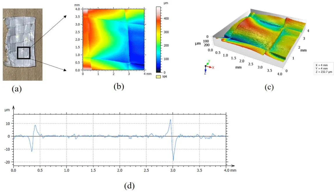
Figure 2 (a) shows the front side of the polystyrene. We define specific region to understand the vertical feature height and the surface roughness of the polystyrene polymer. Figure 2 (b) shows the contour of the defined region having surface area 4 mm by 4 mm. The contour shows the vertical height on the given surface area. The surface profilometer are used to obtain the standard surface roughness and parameters for polymers. Figure 2 (c) shows the 3D plot with the vertical feature height. There are surface heights. Figure 2 (d) shows the surface roughness along the 4 mm length. We obtain the approximate vertical height as 10.78 µm. We consider the value as average surface roughness. The number of points used to calculate the average surface roughness are 5. Table 2 shows the details of the polystyrene. Eq. (1) gives the root mean square value tabulated in table 2. We calculate the surface volume is 16 X 10^-11 m³.

View Figure

Fig. 2

Figure 2 (a) Camera image of the front side of the polystyrene (b) contour from surface profilometer. We consider 4 mm by 4 mm surface area (c) 3D surface profile characteristics (d) line plot to obtain the standard surface roughness parameters in the selected area.

We calculate the the root mean square error (RMSE). The root mean square error is calculated as given in Eq (1).

$RMSE=\sqrt{\frac{1}{n}{\displaystyle \sum }_{i=1}^n{\left(|P_i-O_i|\right)}^2 } \text{ (1)}$

Where p_i is the predicted value, O_i is the actual result for observation i. n is the number of data points.

The steps to calculate the root mean square error are given.

1. We first calculate the residuals (R). The residuals are obtained by calculating the absolute difference between the actual result and the predicted value. We avoid negative values in the answers because they are physical quantities.
2. We calculate the square of the residuals (R²).
3. We calculate the mean squared error (MSE). We sum and mean of all the square of the residuals, respectively. We consider n is the total number of data points.

We calculate the root mean square error by taking the square root of the calculated mean square error.

Standard surface roughness parameters

• Surface roughness R_a

R_a is the most common parameter used in industry. R_a is the average vertical distance that the profile shown in figure 2 (d) deviates from the mean zero line. We use the region of 4 mm to calculate the surface roughness.

$R_a=1/n{{\displaystyle \sum }}_{(i=1)}^n\left|y_i\right|\text{ (2)}$

• where n are the number of data points for the polystyrene polymer of length 4 mm. We consider 60 points. y_i are the vertical distance for each of the 60 points taken from figure 2 (d) using plot digitizer software. We understand the vertical distance in many points are very small <1 um, there are regions at 0.4 mm and 3 mm the vertical distance are > 5 μm. The surface roughness from Eq. (2) results in 3.14 μm. We consider the surface roughness is higher.

Root mean square roughness R_q

The root mean square roughness is calculated using Eq. (3).

$R_q=\sqrt{\frac{1}{n}{\displaystyle \sum }_{i=1}^n{\text{y}}_{\text{i}}^2}\text{ (3)}$

• The root mean square roughness on the front side of the polystyrene polymer is 5.19_um
• Maximum Peak R_p                 
• Maximum peak is the highest point on the surface roughness profile above the mean zero line as shown in figure 2 (d). It is denoted as R_p. The maximum peak surface roughness on the front side of the polystyrene is 12.5
• Maximum Valley R_v
• Maximum valley is the deepest point on the surface roughness profile below the mean zero line as shown in figure 2 (d). It is denoted as . The maximum valley surface roughness on the front side of the polystyrene is -18.25 _um.
• Total height R_t
• The total height is the sum of maximum peak and maximum valley measurements. The total height are calculated using Eq. (4).

$R_t=\left|R_p\right|+\left|R_v\right|\text{ (4)}$

where  is the total height. The total height of the surface roughness on the front side of the polystyrene is 30.75 μm. The surface roughness parameters on the front side of the polystyrene are tabulated in table 3.

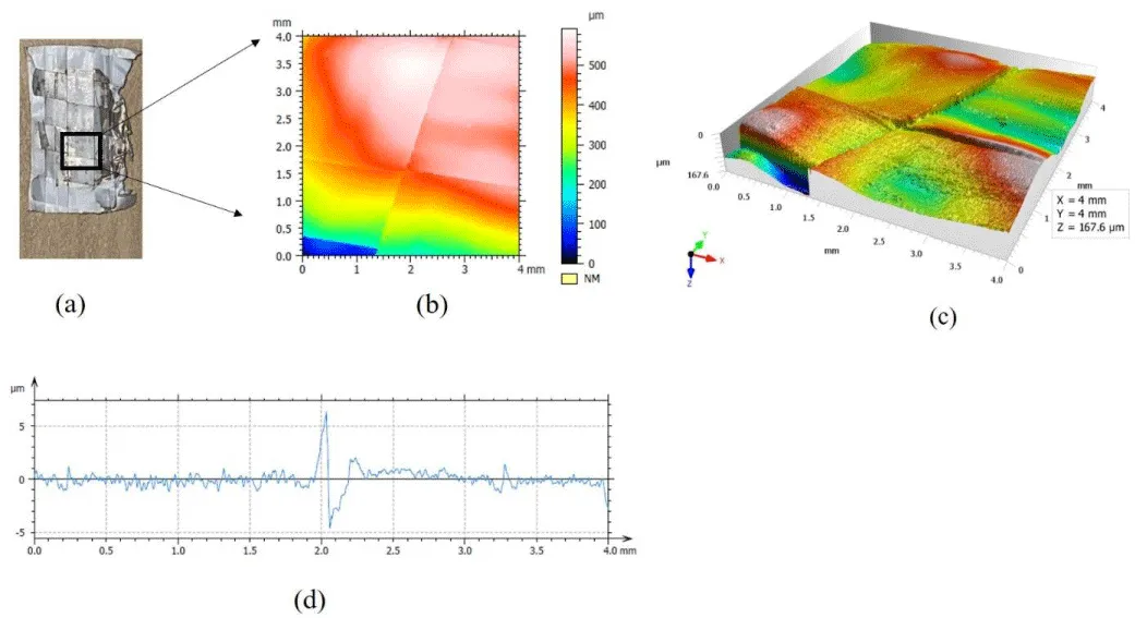
Figure 3 (a) shows the back side of the polystyrene. The back side have small dull color owing to the scanning electron microscopy characterization. The front side of polystyrene are used to obtain the microscopy imaging. We define specific region to understand the vertical height of the back side of the polystyrene. Figure 3 (b) shows the contour in the region. The contour shows the vertical height. Figure 3 (c) shows the 3D plot with the surface uplift visible. Figure 3 (d) shows the surface roughness along the 4 mm length. The 1D, 2D and 3D should be validated with the consistent element model. That is the scope for the future. We obtain the approximate vertical height as 2.5 µm.  Table 4 shows the average surface roughness same as vertical height. The number of points used here are 5. The surface volume is 4 X 10^-11 m³.

View Figure

Fig. 3

Figure 3 (a) Camera image of the back side of the polystyrene after the scanning electron microscopy imaging (b) contour from surface profilometer. We consider 4 mm by 4 mm surface area (c) 3D surface profile characteristics (d) line plot to obtain the standard surface roughness parameters in the selected area.

The average surface roughness on the back side of the polystyrene polymer available in table 4 are 2.5_um . The surface roughness on the back side of the polystyrene are 1_um  The root mean square roughness on the back side of the polystyrene polymer is 1.48_um . The maximum peak surface roughness on the back side of the polystyrene is 6.01_um . The maximum valley surface roughness on the back side of the polystyrene is -4.3_um . The total height of the surface roughness on the back side of the polystyrene is 10.31_um . The standard surface roughness parameters of polystyrene are given in table 3.

Figure 4 (a) shows the polyethylene oxide. Figure 4 (b) shows the 1 µm (c) 2 µm (d) 4 µm (e) 10 µm, (f) 20 µm, (g) 100 µm and (h) 200 µm resolution. Figure 4 (i) shows the materials present in the polyethylene oxide. The materials are carbon and oxygen. The composition of carbon is 68.2% and oxygen is 31.8 %. The relation with the advanced new camera having microscopy features with the elements studied in this paper needs further theory.

View Figure

Fig. 4

Figure 4 (a) Camera image of the actual transparent polyethylene oxide. Scanning electron microscopy imaging (b) 1 µm (c) 2 µm (d) 4 µm (e) 10 µm (f) 20 µm (g) 100 µm (h) 200 µm resolution and (i) energy dispersive spectroscopy to obtain the chemical elements in the transparent polyethylene oxide. The composition of carbon is 68.2 % and oxygen 31.8 %.

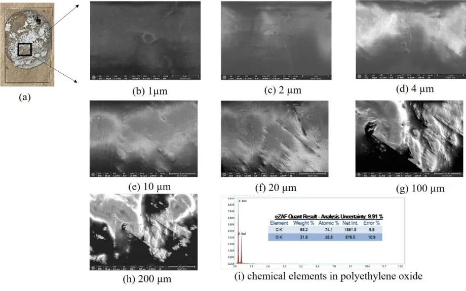
Figure 5 (a) shows the non-coated transparent polyethylene oxide. The non-coated by definition are the top surface that are used in the scanning electron microscopy machine. The coated regions are different. The coated regions are dull because they are resting with direct contact on the microscopy machine. To the non-coated transparent polyethylene oxide we define specific region to understand the vertical feature. Figure 5 (b) shows the contour in the given region. The contour length is 4 mm and width is 4 mm. The contour shows the vertical height. Figure 5 (c) shows the 3D plot that have the ridges by definition some surface roughness regions. Figure 5 (d) shows the 1D line plot of the surface roughness along the 4 mm. We approximate the vertical height as 36.7 µm.  The surface volume is  5.9×10−10m³.

View Figure

Fig. 5

Figure 5 (a) Camera image of the non coated side of the transparent polyethylene oxide (b) contour from surface profilometer. We consider 4 mm by 4 mm surface area (c) 3D surface profile characteristics (d) line plot to obtain the standard surface roughness parameters in the selected area.

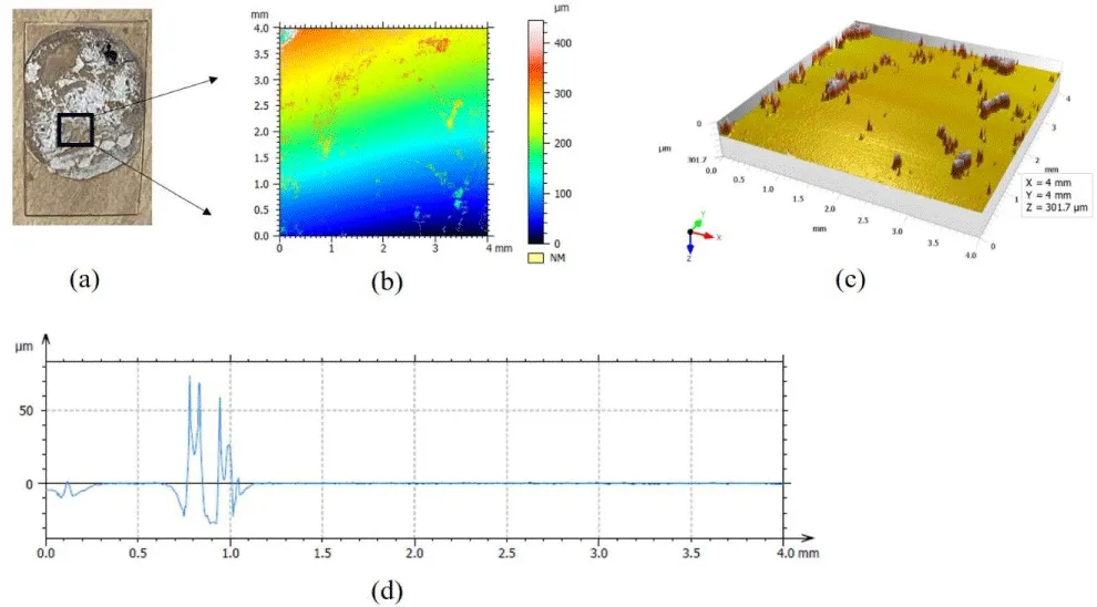
Table 5 shows the average roughness is 37.6  μm. We believe the distance of objects and shape can be obtained from our polymer based sensor study. Table 3 shows the surface roughness for non-coated transparent polyethylene oxide.  The table 3 reads the surface roughness on the non-coated side of the polyethylene oxide are 14.98 μm.  The root mean square roughness is 24.41 μm. The maximum peak surface roughness is 71.3 μm. The maximum valley surface roughness is -26.67 μm. The total height of the surface roughness on the non-coated side of the polyethylene oxide is 97.97 μm. Figure 6 (a) shows the coated side of the polyethylene oxide. We define specific region to understand the vertical height. Figure 6 (b) shows the contour. The contour length is 4 mm and width is 4 mm. The contour shows the vertical height. Figure 6 (c) shows the 3D plot. We observe the ridges at many instances. Figure 6 (d) shows the surface roughness along the 4 mm length. We approximate the vertical height as 6.7 µm.  We calculate the surface volume is 1.1 X 10^-10 m³.

View Figure

Fig. 6

Figure 6 (a) Camera image of the coated side of the transparent polyethylene oxide after the scanning electron microscopy imaging (b) contour from surface profilometer. We consider 4 mm by 4 mm surface area (c) 3D surface profile characteristics (d) line plot to obtain the standard surface roughness parameters in the selected area.

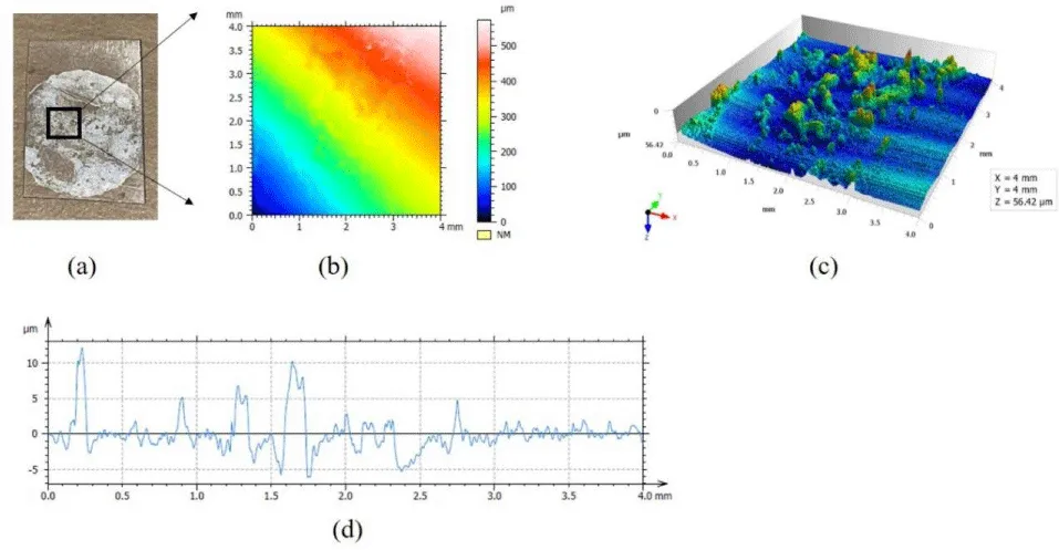
Table 6 shows the vertical height on the coated side of the transparent polyethylene oxide.  We consider 5 points. The average surface roughness are 6.7 μm. The surface roughness are 2.45 μm The root mean square roughness are 3.46 μm. The maximum peak surface roughness are 11.78 μm. The maximum valley surface roughness is -6.01 μm. The total height of the surface roughness on the coated side of the polyethylene oxide are 17.79 μm.

Figure 7 (a) shows the translucent polyethylene oxide (b) 500 nm and (c) 5 µm resolution. Figure 7 (d) shows the materials present in the translucent polyethylene oxide. The materials in the translucent polyethylene oxide are carbon, oxygen, sodium, aluminum, silicon and chlorine. The composition of carbon is 98.2%, oxygen is 1.3 %, sodium 0.2%, aluminum 0.1 %, silicon 0.1 % and chlorine 0.1 %, respectively.

View Figure

Fig. 7

Figure 7 (a) Camera image of the actual translucent polyethylene oxide. Scanning electron microscopy imaging (b) 500 nm (c) 5 µm resolution and (i) energy dispersive spectroscopy to obtain the chemical elements in the translucent polyethylene oxide. The composition of carbon is 98.2 %, oxygen 1.3 %, sodium 0.2 %, aluminum 0.1 %, silicon 0.1 % and chlorine is 0.1 %.

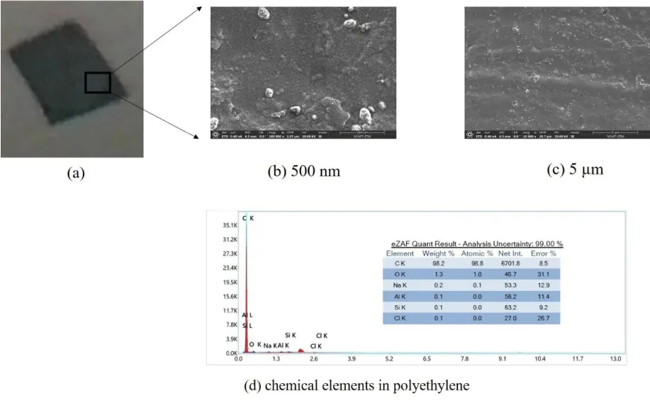
Figure 8 (a) shows the non-coated side of the translucent polyethylene oxide. The non coated region are used to image in the microscopy. The coated region is the resting surface during microscopy imaging. We define specific region to understand the vertical height. Figure 8 (b) shows the contour. The length of the contour is 4 mm and width is 4 mm. The contour shows the vertical height. Figure 8 (c) shows the 3D plot with ridge waves. Figure 8 (d) shows the 1D along the 4 mm line plot of the surface roughness. The surface volume is 1.1×10−11m³ . We approximate the vertical height as 0.68 µm.

View Figure

Fig. 8

Figure 8 (a) Camera image of the non coated side of the translucent polyethylene oxide (b) contour from surface profilometer. We consider 4 mm by 4 mm surface area (c) 3D surface profile characteristics (d) line plot to obtain the standard surface roughness parameters in the selected area.

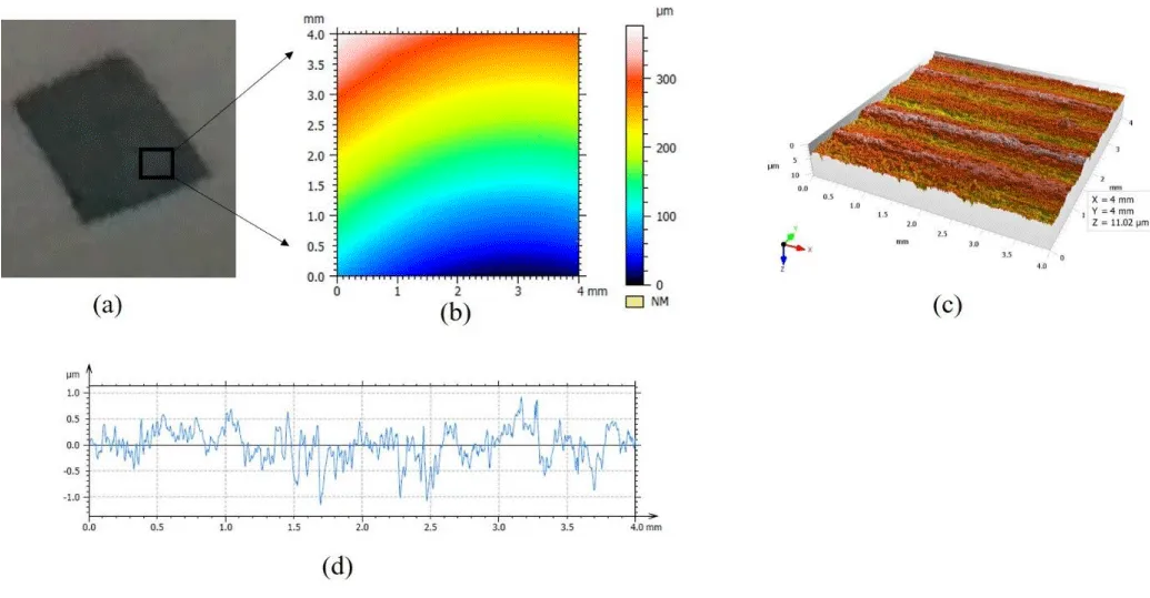
Table 7 shows the average surface roughness same as vertical height. We consider 5 points to obtain the average surface roughness. The value is 0.68 μm. Table 3 shows the surface roughness parameters. The surface roughness of the non-coated polyethylene oxide are 0.32  The root mean square roughness is 0.39 μm. The maximum peak surface roughness is 0.86 μm. The maximum valley surface roughness is -1.08 μm. The total height of the surface roughness on the non coated side of the translucent polyethylene oxide is 1.94 μm. Figure 9 (a) shows the coated side of the translucent polyethylene oxide. We define specific region to understand the vertical height. Figure 9 (b) shows the contour in the region. The contour size have length 4 mm and width 4 mm. The contour shows the vertical height. Figure 9 (c) shows the 3D plot with surface heights. Figure 9 (d) shows the surface roughness along the 4 mm length. We approximate the vertical height as 4.53 µm.  We calculate the surface volume is 7.25 X 10^-11 m³.

View Figure

Fig. 9

Figure 9 (a) Camera image of the coated side of the translucent polyethylene oxide after the scanning electron microscopy imaging (b) contour from surface profilometer. We consider 4 mm by 4 mm surface area (c) 3D surface profile characteristics (d) line plot to obtain the standard surface roughness parameters in the selected area.

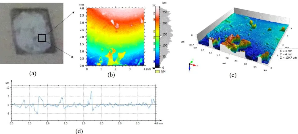
Table 8 shows the average surface roughness is 4.53 µm. Table 3 shows the surface roughness of the coated polyethylene oxide are 1.58 μm The root mean square roughness is 2.1 μm. The maximum peak surface roughness is 7.27 μm. The maximum valley surface roughness is -5.25 μm. The total height of the surface roughness on the coated side of the translucent polyethylene oxide is 12.52 μm.

Figure 10 (a) shows the polyvinyl chloride. Figure 10 (b) shows the 500 nm and (c) 5 µm imaging resolution. Figure 10 (d) shows the materials present in the polyvinyl chloride. The composition of carbon is 57.8 %, oxygen is 6.5 %, magnesium 0.3 %, aluminum 0.2 %, silicon 0.3 %, chlorine 28.2 %, calcium 4.1 %, titanium 0.6 % and molybdenum 1.8 %, respectively. 

View Figure

Fig. 10

Figure 10 (a) Camera image of the actual polyvinyl chloride. Scanning electron microscopy imaging (b) 500 nm (c) 5 µm resolution and (i) energy dispersive spectroscopy to obtain the chemical elements in the polyvinyl chloride. The composition of carbon is 57.8 %, oxygen 6.5 %, magnesium 0.3 %, aluminum 0.2 %, silicon 0.3 %, chlorine 28.2 %, calcium 4.1 %, titanium 0.6 % and molybdenum 1.8 %.

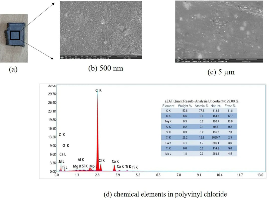
Figure 11 (a) shows the front side of the polyvinyl chloride. The front side is used to image in the microscopy. We define specific region to understand the vertical height. Figure 11 (b) shows the contour. The contour length is 4 mm and width is 4 mm. The contour shows the vertical height. Figure 11 (c) shows the 3D plot to understand the surface roughness. Figure 11 (d) shows the 1D line plot along the 4 mm to observe the surface roughness. The surface volume is 1.1×10−11m³. We approximate the vertical height as 0.68 µm.

View Figure

Fig. 11

Figure 11 ((a) Camera image of the front side of the polyvinyl chloride (b) contour from surface profilometer. We consider 4 mm by 4 mm surface area (c) 3D surface profile characteristics (d) line plot to obtain the standard surface roughness parameters in the selected area.

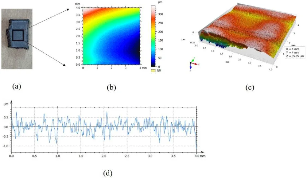
Table 9 shows the average surface roughness same as the vertical feature is 0.68 μm. Table 3 shows the surface roughness is 0.28 μm The root mean square roughness is 0.34 μm. The maximum peak surface roughness is 0.79 μm. The maximum valley surface roughness is -0.74 μm. The total height of the surface roughness on the front side of the polyvinyl chloride is 1.53 μm. Figure 12 (a) shows the back side of the polyvinyl chloride. The back side becomes coated side because the back side of the polyvinyl chloride are the resting side during the microscopy. The front side is used to image. We define specific region to understand the vertical height. Figure 12 (b) shows the contour. The contour have length 4 mm and width 4 mm. The contour shows the vertical height with shades. Figure 12 (c) shows the 3D plot. They have surface heights. Figure 12 (d) shows the surface roughness along the 4 mm length. The surface volume is 7.6×10−11 m³. We approximate the vertical height as 4.76 µm.

View Figure

Fig. 12

Figure 12 (a) Camera image of the back side of the polyvinyl chloride after the scanning electron microscopy imaging (b) contour from surface profilometer. We consider 4 mm by 4 mm surface area (c) 3D surface profile characteristics (d) line plot to obtain the standard surface roughness parameters in the selected area.

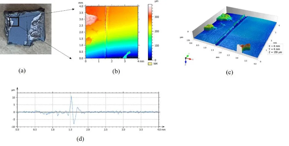
Table 10 shows the average surface roughness is 4.76 µm. Table 3 shows the surface roughness parameters. The surface roughness of the back side of the polyvinyl chloride is 1.38 μm The root mean square roughness is 2.4 μm. The maximum peak surface roughness is 10.32 μm. The maximum valley surface roughness is -7.9 μm. The total height of the surface roughness on the back side of the polyvinyl chloride is 18.22 μm. Here, we study textile cloth. We print the textile cloth with image. Figure 13 (a) shows the cloth polymer. The textile have print and non-print regions. We analyze the non-print region of the cloth. Figure 13 (b) shows the 5 µm (c) 10 µm (d) 30 µm (e) 50 µm (f) 100 µm (g) 300 µm and (h) 500 µm resolution. Figure 13 (i) shows the materials present in the non-printed cloth. The materials are carbon, oxygen and copper. The composition of carbon is 74.7%, oxygen 15 % and copper 10.3 %. We observe distinct fibres and coils closely packed in the non-print area.

View Figure

Fig. 13

Figure 13 (a) Camera image of the textile cloth. We consider non print white region. Scanning electron microscopy with image resolution (b) 5 µm (c) 10 µm (d) 30 µm (e) 50 µm (f) 100 µm (g) 300 µm (h) 500 µm and (i) energy dispersive spectroscopy to obtain the chemical elements in the white region of cloth. The composition of carbon is 74.7 %, oxygen 15 % and copper 10.3 %.

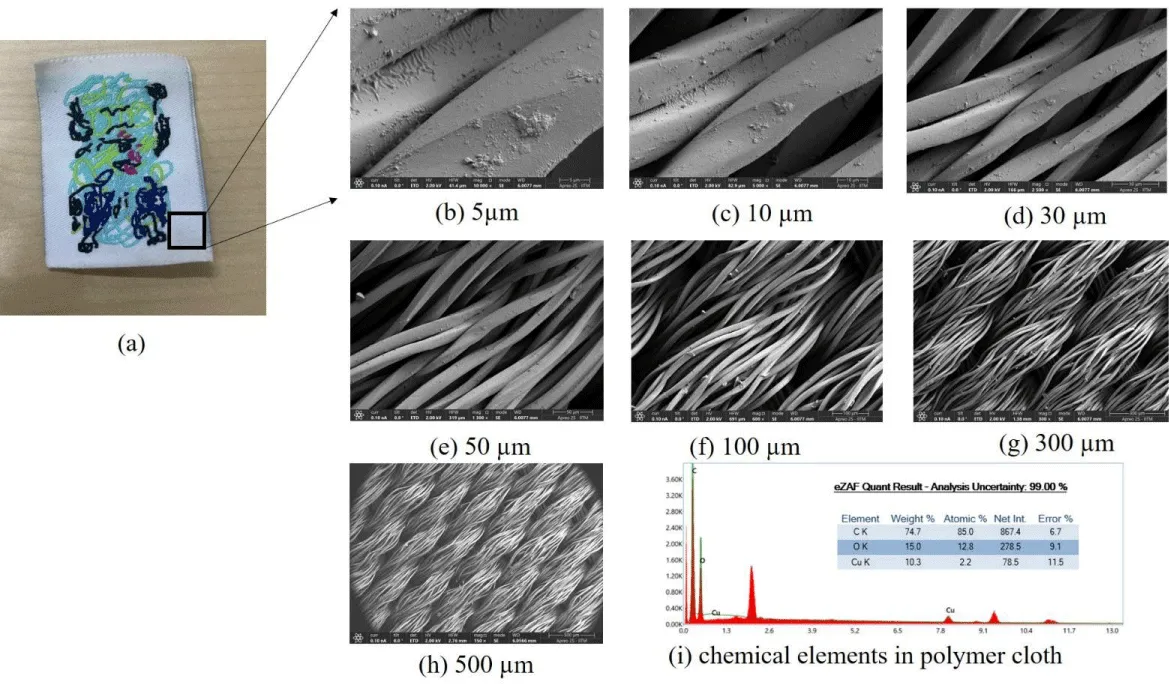
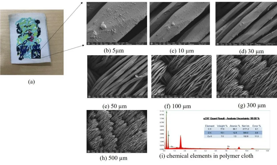
Figure 14 (a) shows the printed region in the textile cloth. Figure 14 (b) shows the imaging in the printed region for 5 µm (c) 10 µm, (d) 30 µm, (e) 50 µm, (f) 100 µm, (g) 300 µm and (h) 500 µm resolution. Figure 14 (i) shows the materials present in the printed area of the cloth. The materials are carbon, oxygen and copper. The composition of carbon is 77.9%, oxygen 15.1 % and copper 7 %. We observe the difference of the structure in the print portion of the textile. We observe many fibres and coils with density arrangement prominent compared to the non-printed cloth region. Table 11 shows the different polymers and their chemical elements with the composition. The polymers are front and back side of the polystyrene. We study coated and non-coated transparent polyethylene oxide, translucent polyethylene oxide and polyvinyl chloride. We study non print and print region on the textile cloth. 

View Figure

Fig. 14

Figure 14 (a) Camera image of the textile cloth. We consider print indicated region. Scanning electron microscopy with image resolution (b) 5 µm (c) 10 µm (d) 30 µm (e) 50 µm (f) 100 µm (g) 300 µm (h) 500 µm and (i) energy dispersive spectroscopy to obtain the chemical elements in the print region of the cloth. The composition of carbon is 77.9 %, oxygen 15.1 % and copper 7 %.

Polystyrene exhibits average surface roughness of 10.78 µm on its front side and 2.5 µm on its back side. The molecular state of polystyrene provides the smooth structure during its usage. The surface roughness of the transparent polyethylene oxide is 36.7 . They have high surface roughness due to the preparation process of add the color. There could also be material consistency during the color addition to produce the transparent polyethylene oxide.  The consistency in the preparation process resulted in low surface roughness in the translucent polyethylene oxide. The polymer chains in the translucent polyethylene oxide are packed together tightly and evenly. The polyvinyl chloride material is prepared using additive manufacturing process. Polyvinyl chloride are used in plumbing and housing pipes, which require highly uniform and smooth surfaces for efficient fluid transport and insulation. The surface roughness in the textile cloth are driven by the fibrous geometry. The printed areas show more prominent arrangements of fibres and coils, suggesting that the addition of print material changes the gaps in the fabric. Thus, we observe surface roughness in the printed material cloth region in the measuremen

Conclusion

To conclude we study polymers that include polystyrene, transparent polyethylene oxide, translucent polyethylene oxide, polyvinyl chloride and cloth. The cloth have print image on them. We use surface profilometer machine, scanning electron microscopy and energy dispersive spectroscopy. The surface profilometer provides the standard surface roughness parameters to our polymers. The imaging are done using microscopy. The chemical elements and their composition are obtained in our study. The predict ability of the element composition in polymers using neural networks are scope for the future. We studied the density and structure on cloth with print images. Our work can find applications in sensors, geometry finding to materials, packaging, automobiles, pipe flow, coatings and printers.

Acknowledgment

There is no funding for this work.

Author contributions

Nandigana V. R. Vishal: Conceptualization, Data curation, Formal analysis, investigation, methodology, resources, software, supervision, validation, visualization, writing – original draft, writing – review and editing.

Conflicts of interest

The authors declare no conflict of interest.

Data availability

The data from the current study are available from the corresponding author upon reasonable request.