Analysis and Control of Alzheimer's Disease Models

Millions of people are affected by Alzheimer's disease, which is a progressive neurodegenerative disorder. It is important to understand the progression dynamics of this disease to be able to minimize the damage that is caused by it. This article provides a mathematical framework to develop strategies to slow down the progression of Alzheimer's disease. Bifurcation analysis is a powerful mathematical tool used to deal with the nonlinear dynamics of any process. Several factors must be considered, and multiple objectives must be met simultaneously. Bifurcation analysis and Multiobjective Nonlinear Model Predictive Control (MNLMPC) calculations are performed on two Alzheimer’s disease models. The MATLAB program MATCONT was used to perform the bifurcation analysis. The MNLMPC calculations were performed using the optimization language PYOMO in conjunction with the state-of-the-art global optimization solvers IPOPT and BARON. The bifurcation analysis revealed the existence of limit points in the models. The limit points were beneficial because they enabled the multiobjective nonlinear model predictive control calculations to converge to the Utopia point in both problems, which is the most beneficial solution. A combination of bifurcation analysis and multiobjective nonlinear model predictive control for Alzheimer’s disease models is the main contribution of this paper.

Chao CC, et al. [1] discussed the transforming growth factor beta in Alzheimer’s disease. Lue LF, et al. [2] showed that the soluble amyloid beta peptide concentration is a predictor of synaptic change in Alzheimer's disease. Mehta PD, et al. [3] investigated the plasma and cerebrospinal fluid levels of amyloid β proteins 1-40 and 1-42 in Alzheimer disease. Penkowa M, et al. [4] showed the impaired inflammatory response and increased oxidative stress and neurodegeneration after brain injury in interleukin-6-deficient mice. Penkowa M, et al. [5] demonstrated that the Interleukin-6 deficiency reduces the brain inflammatory response and increases oxidative stress and neurodegeneration after kainic acid-induced seizures. Wyss-Coray T, et al. [6] showed that TGF-β1 promotes microglial amyloid-β clearance and reduces plaque burden in transgenic mice. Jacobsen JS, et al. [7], investigated the early-onset behavioural and synaptic deficits in a mouse model of Alzheimer's disease. Wyss-Coray T. [8] showed that the TGF-β pathway was a potential target in neurodegeneration and Alzheimer’s disease. Das P, et al. [9] demonstrated the dysfunction of TGF-β signaling in Alzheimers disease. Tobinick E, et al. [10] used the TNF-alpha modulation for treatment of Alzheimer’s disease. Green KN, et al. [11], investigated the role of calcium in the pathogenesis of Alzheimer's disease and transgenic models. Lyketsos CG, et al. [12] showed that naproxen and celecoxib do not prevent AD in early results from a randomized controlled trial. Town T, et al. [13] demonstrated that. blocking TGF-β–smad2/3 innate immune signaling mitigates Alzheimer-like pathology. Cheung KH, et al. [14], illustrated the mechanism of Ca2+ disruption in Alzheimer's disease by presenilin regulation of InsP3 receptor channel gating. Bezprozvanny I, et al. [15] researched the neuronal calcium mishandling and the pathogenesis of Alzheimer's disease. Bojarski L, et al. [16] investigated the calcium dysregulation in Alzheimer's disease. Martin BK, et al. [17] researched the cognitive function over time in the Alzheimer ’s disease and produced results of a randomized, controlled trial of naproxen and celecoxib.

Lopez JR, et al. [18] Increased intraneuronal resting [Ca2+] in adult Alzheimer's disease mice. Nelson O, et al. [19], investigated familial Alzheimer's disease mutations in presenilins and studied the effects on endoplasmic reticulum calcium homeostasis and correlation with clinical phenotypes. Puri IK, et al. [20], studied Mathematical models for the pathogenesis of Alzheimer's disease. Berridge MJ. [21] Tested the calcium hypothesis of Alzheimer's disease. Imbimbo BP, et al. [22] investigated whether NSAIDs are useful to treat Alzheimer’s disease or mild cognitive impairment. Berridge MJ. [23] studied the effect of calcium signalling on Alzheimer's disease. Anastasio TJ. [24] performed data-driven modelling of Alzheimer's disease pathogenesis. Camandola S, et al. [25] studied the aberrant subcellular neuronal calcium regulation in aging and Alzheimer's disease. Ho M, et al. [26] showed that the effects of metal chelators on γ-secretase indicate that calcium and magnesium ions facilitate cleavage of Alzheimer's amyloid precursor substrate. Itkin A, et al. [27], demonstrated that calcium ions promote the formation of amyloid b-peptide (1-40) oligomers causally implicated in neuronal toxicity of Alzheimer's disease. Müller M, et al. [28] studied the constitutive cAMP response element binding protein (CREB) activation by Alzheimer's disease presenilin-driven inositol trisphosphate receptor (InsP3R) Ca2+ signaling.

Schmidt V, et al. [29] performed quantitative modelling of amyloidogenic processing and its influence by SORLA in Alzheimer's disease. Ma T, et al. [30] studied mitochondrial modulation of store-operated Ca2+ entry in model cells of Alzheimer's disease. Woods NK, et al. [31] studied the effect of neuronal calcium signaling on Alzheimer's disease. De Kimpe L, et al. [32] showed that disturbed Ca2+ homeostasis increases glutaminyl cyclase expression, connecting two early pathogenic events in Alzheimer's disease in vitro. Berridge MJ. [33] investigated the dysregulation of neural calcium signaling in Alzheimer's disease. Cabezas I, et al. [34] investigated the role of glial cells in Alzheimer's disease. Chen JH, et al. [35] studied strategies involving protection of TGF-β1 against neuroinflammation and neurodegeneration in Aβ1–42-induced Alzheimer’s disease in model rats. Von Bernhardi R, et al. [36] studied the role of TGFβ signaling in the pathogenesis of Alzheimer’s disease. Bertsch M, et al. [37] and Hao W, et al. [38] developed mathematical models for the onset and progression of Alzheimer’s disease. Forloni G, et al. [39] performed research involving oligomers and inflammation in Alzheimer’s disease.

Kinney JW, et al. [40] conclude that inflammation is a central mechanism in Alzheimer’s disease. Zhu M, et al. [41] investigated whether inflammation be resolved in Alzheimer’s disease. Ozben T, et al. [42] studied neuro-inflammation and anti-inflammatory treatment options for Alzheimer’s disease. Ali MM, et al. [43] provide recommendations for anti-inflammatory treatments in Alzheimer’s disease. Ciuperca IS, et al. [44] developed an in vitro mathematical model involving Alzheimer's disease and prions. Andrade-Restrepo M, et al. [45] modelled the spatial propagation of Aβ oligomers in Alzheimer’s disease. Rivers-Auty J, et al. [46] investigated the use of anti-inflammatories in Alzheimer’s disease-potential therapy. Huang LK, et al. [47] performed clinical trials of new drugs for Alzheimer's disease. Li H, et al. [48] developed a mathematical model of Alzheimer’s disease with prion proteins interactions and treatment. Hu J, et al. [49] performed optimal control calculations of a stochastic reaction diffusion model for Alzheimer’s disease with impulse and time-varying delay. Hao W, et al. [50] developed a strategy for optimal anti-amyloid-beta therapy for Alzheimer’s disease via a personalized mathematical model. Al-Ghraiybah NF, et al. [51] studied glial cell-mediated neuroinflammation in Alzheimer’s disease. Pal S, et al. [52] modelled Anti-amyloid-Beta Therapy for Alzheimer’s Disease. Van Dyck CH, et al. [53] investigated Lecanemab in early Alzheimer’s disease. Ciuperca I, et al. [54] performed a qualitative analysis of an A β-monomer model with inflammation processes for Alzheimer’s disease. Caluwé J, et al. [55] discuss he progression towards Alzheimer's disease described as a bistable switch arising from the positive loop between amyloids and Ca2+.

Torres N, et al. [56], performed optimal control calculations involving anti-inflammatory treatments of Alzheimer’s disease. All the optimal control work involving Alzheimer’s disease involved single-objective optimal control. In this article we perform multiobjective nonlinear model predictive control in conjunction with bifurcation analysis for two Alzheimer’s disease. The work Caluwé J, et al. [55] and Ciuperca I, et al. [54] capture analytically the dynamics of the Alzheimer’s disease models and represent theoretically most of the features and hence these two models will be used for the calculations in this paper. These models will be referred to as model 1 and model 2. This paper is organized as follows. First, the Alzheimer’s disease models are presented. The numerical procedures (Bifurcation analysis and Multiobjective Nonlinear Model Predictive Control (MNLMPC) are then described. This is followed by the results and discussion and conclusions.

Model 1

The model equations are

$\begin{array}{l}\frac{da}{dt}=v_1-k_{1}a+\frac{v_{\alpha }(c^n)}{((k_{\alpha }{}^n)+(c^n))};\text{ (1)}\\ \frac{dc}{dt}=v2-(k_{2}c)+k_{\beta }(a^m);\end{array}$

The parameter values are

$\begin{array}{l}{v}_{\alpha }=0.05;k_{\alpha }=120;n=2;k_1=0.01;\\ k_{\beta }=0.2;m=4;k_2=0.1;\end{array}$

a and c represent the concentrations of Aβ and the intracellular Ca2+. $v_1,v_2$ represent the synthesis rate of Aβ and the rate at which Ca2+ enters the cytoplasm. These are the bifurcation and control parameters, respectively.

Model 2

The model equations are

$\begin{array}{l}\frac{db}{dt}=r_1{(}^m-{\gamma }_0(b)\\ \frac{d{b}_p}{dt}={\gamma }_0(b)-{\tau }_p{b}_p\\ \frac{d(mval)}{dt}=\frac{{\tau }_S(ival)}{(1+(c(b^{nval}))}-d(mval)-r_2(b)mval-r_1{(}^m\text{ (2)}\\ \frac{d(mcap)}{dt}=\frac{{\alpha }_{1}b(mcap)\left(\stackrel{⌢}{m}-mcap\right) }{\left(1+\left({\alpha }_{2}b\right)\right)} -sigma(mcap)-{\lambda }_M\\ \frac{d(ival)}{dt}=\frac{{\tau }_{1}b(mcap)}{\left(1+\left({\tau }_{2}b\right)\right)}-{\tau }_3(ival)\end{array}$

The parameter values are

$\begin{array}{l}{r}_1=0.1;r_2=0.1;{\gamma }_0={0.0}_{}5;{\tau }_1=1;\\ {\tau }_2=1;{\tau }_3=1;{\tau }_p=0.03;{\tau }_s=1;c=1;\\ nval=2;{\alpha }_1=1;{\alpha }_2=1;{\lambda }_M=1.e-03;\text{ <mover accent="true"> m <mo>⌢</mo> </mover>}=1;\end{array}$

b and bp represent the oligomer concentration and the concentration of oligomers in plaques. mval and mcap represent the monomer and microglial cell concentrations. ival represents the interleukin concentration. Sigma and d are the degradation rates of microglial cells and the degradation rate of monomers. These are the bifurcation and control parameters, respectively.

The MATLAB software MATCONT is used to perform the bifurcation calculations. Bifurcation analysis deals with multiple steady-states and limit cycles. Multiple steady states occur because of the existence of branch and limit points. Hopf bifurcation points cause limit cycles. A commonly used MATLAB program that locates limit points, branch points, and Hopf bifurcation points is MATCONT (Dhooge A, et al. [57]; Dhooge A, et al. [58]). This program detects Limit Points (LP), Branch Points(BP), and Hopf bifurcation points(H) for an ODE system

$\frac{dx}{dt}=f(x,\alpha )\text{ (3)}$

$x\in R^n$ Let the bifurcation parameter be Since the gradient is orthogonal to the tangent vector,

The tangent plane at any point $w=[w_1,w_2,w_3,w_4,\mathrm{....}{w}_{n+1}]$ must satisfy

$Aw=0\text{ (4)}$

where A is

$A=[\partial f/\partial x|\partial f/\partial \alpha ]\text{ (5)}$

where $\partial f/\partial x$ is the Jacobian matrix. For both limit and branch points, the matrix $[\partial f/\partial x]$ must be singular. The n+1 th component of the tangent vector $w_{n+1}$ = 0 for a limit point (LP)and for a branch point (BP) the matrix $\left[\begin{array}{l}A\\ w^T\end{array}\right]$ must be singular. At a Hopf bifurcation point,

$\det (2f_x(x,\alpha )@I_n)=0\text{ (6)}$

@ indicates the bialternate product while $I_n$ is the n-square identity matrix. Hopf bifurcations cause limit cycles and should be eliminated because limit cycles make optimization and control tasks very difficult. More details can be found in Kuznetsov YA. [59]; Kuznetsov YA. [60]) and Govaerts WJF. [61].

Flores TA, et al. [62] developed a Multiobjective Nonlinear Model Predictive Control (MNLMPC) method that is rigorous and does not involve weighting functions or additional constraints. This procedure is used for performing the MNLMPC calculations. Here ${\displaystyle \sum _{t_{i=0}}^{t_i=t_f}{q}_j(t_i)}$ (j=1, 2..n) represents the variables that need to be minimized/maximized simultaneously for a problem involving a set of ODE

$\frac{dx}{dt}=F(x,u)\text{ (7)}$

$t_f$ being the final time value, and n the total number of objective variables and . u the control parameter. This MNLMPC procedure first solves the single objective optimal control problem independently optimizing each of the variables ${\displaystyle \sum _{t_{i=0}}^{t_i=t_f}{q}_j(t_i)}$ individually. The minimization/maximization of ${\displaystyle \sum _{t_{i=0}}^{t_i=t_f}{q}_j(t_i)}$ will lead to the values $q_j^{*}$ . Then the optimization problem that will be solved is

$\begin{array}{l}\min ({\displaystyle \sum _{j=1}^n({\displaystyle \sum _{t_{i=0}}^{t_i=t_f}{q}_j(t_i)}-q_j^{*}){)}^2}\\ subjectto\frac{dx}{dt}=F(x,u);\text{ (8)}\end{array}$

This will provide the values of u at various times. The first obtained control value of u is implemented and the rest are discarded. This procedure is repeated until the implemented and the first obtained control values are the same or if the Utopia point where ( ${\displaystyle \sum _{t_{i=0}}^{t_i=t_f}{q}_j(t_i)}=q_j^{*}$ for all j) is obtained.

Pyomo Hart WE, et al. [63] is used for these calculations. Here, the differential equations are converted to a Nonlinear Program (NLP) using the orthogonal collocation method The NLP is solved using IPOPT Wächter A, et al. [64] and confirmed as a global solution with BARON Tawarmalani M, et al.[65].

The steps of the algorithm are as follows

Optimize ${\displaystyle \sum _{t_{i=0}}^{t_i=t_f}{q}_j(t_i)}$ and obtain $q_j^{*}$ at various time intervals ti. The subscript i is the index for each time step.

Minimize $({\displaystyle \sum _{j=1}^n({\displaystyle \sum _{t_{i=0}}^{t_i=t_f}{q}_j(t_i)}-q_j^{*}){)}^2}$ and get the control values for various times.

Implement the first obtained control values

Repeat steps 1 to 3 until there is an insignificant difference between the implemented and the first obtained value of the control variables or if the Utopia point is achieved. The Utopia point is when ${\displaystyle \sum _{t_{i=0}}^{t_i=t_f}{q}_j(t_i)}=q_j^{*}$ for all j.

Sridhar LN. [66] proved that the MNLMPC calculations to converge to the Utopia solution when the bifurcation analysis revealed the presence of limit and branch points. This was done by imposing the singularity condition on the co-state equation [67]. If the minimization of $q_1$ lead to the value $q_1^{*}$ and the minimization of $q_2$ lead to the value $q_2^{*}$ The MNLPMC calculations will minimize the function ${(q_1-q_1^{*})}^2+{(q_2-q_2^{*})}^2$ . The multiobjective optimal control problem is

$\begin{array}{l}\min {(}^{q_1}+{(}^{q_2}subjectto\frac{dx}{dt}=F(x,u)\text{ (9)}\\ \end{array}$

Differentiating the objective function results in

$\begin{array}{l}\frac{d}{d{x}_i}({(}^{q_1}+{(}^{q_2})=\\ 2(q_1-q_1^{*})\frac{d}{d{x}_i}(q_1-q_1^{*})+2(q_2-q_2^{*})\frac{d}{d{x}_i}(q_2-q_2^{*})\text{ (10)}\end{array}$

The Utopia point requires that both $(q_1-q_1^{*})$ and $(q_2-q_2^{*})$ are zero. Hence

$\frac{d}{d{x}_i}({(q_1-q_1^{*})}^2+{(q_2-q_2^{*})}^2)=0\text{ (11)}$

the optimal control co-state equation (Upreti; 2013) is

$\frac{d}{dt}({\lambda }_i)=-\frac{d}{d{x}_i}({(q_1-q_1^{*})}^2+{(q_2-q_2^{*})}^2)-f_x{\lambda }_i;{\lambda }_i(t_f)=0\text{ (12)}$

${\lambda }_i$ is the Lagrangian multiplier. $t_f$ is the final time. The first term in this equation is 0 and hence

$\frac{d}{dt}({\lambda }_i)=-f_x{\lambda }_i;{\lambda }_i(t_f)=0\text{ (13)}$

At a limit or a branch point, for the set of ODE $\frac{dx}{dt}=f(x,u)$ $f_x$ is singular. Hence there are two different vectors-values for $[{\lambda }_i]$ where $\frac{d}{dt}({\lambda }_i)>0$ and $\frac{d}{dt}({\lambda }_i)<0$ . In between there is a vector $[{\lambda }_i]$ where $\frac{d}{dt}({\lambda }_i)=0$ . This coupled with the boundary condition ${\lambda }_i(t_f)=0$ will lead to $[{\lambda }_i]=0$ . This makes the problem an unconstrained optimization problem, and the only solution is the Utopia solution.

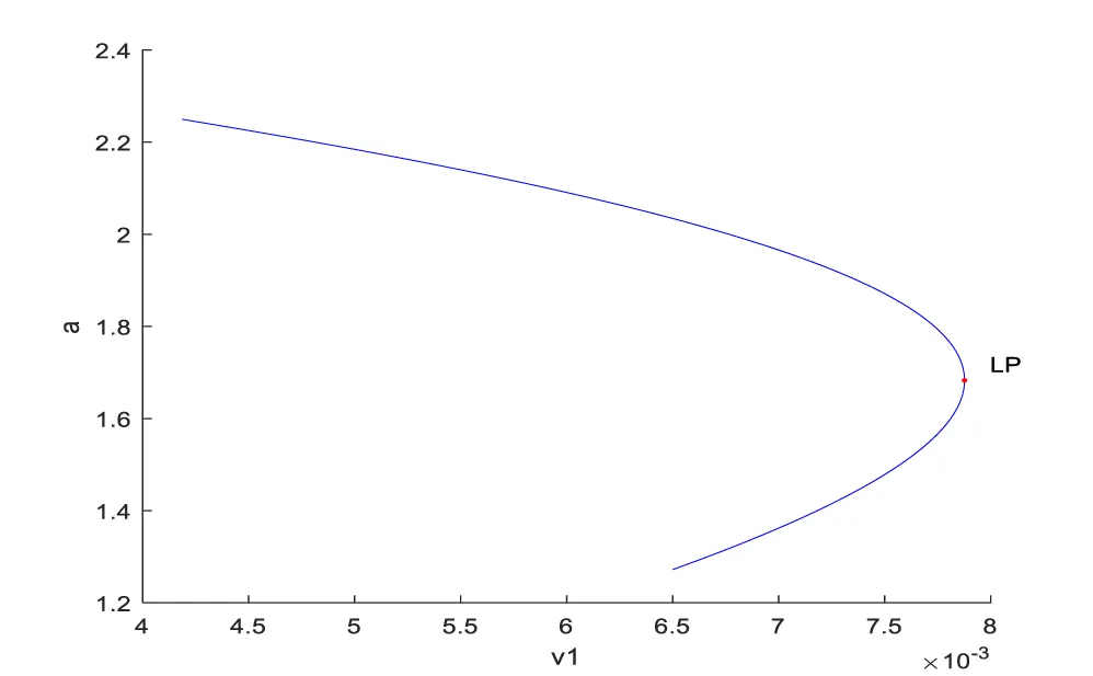
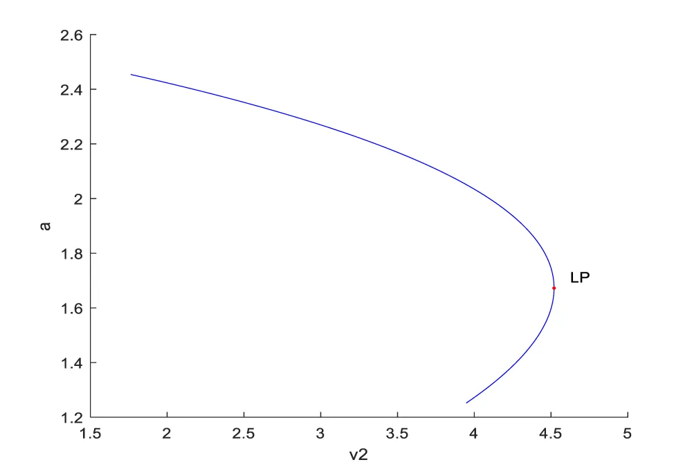
Bifurcation analysis for model 1 revealed the existence of limit points for both the bifurcation parameters v1 and v2. The coordinates for the 2 limit points are (a,c,v1)=( 1.682845, 56.040073, 0.007876) and (a,c,v2)=( 1.672121, 60.828416, 4.519333 ). These limit points are shown in figures 1a,b. The limit points cause the profiles to change direction and this is shown in the figures.

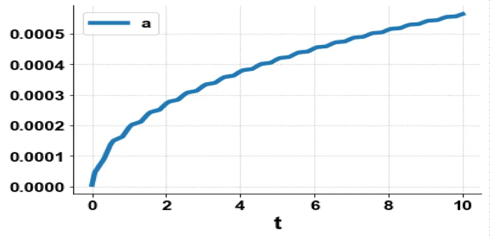
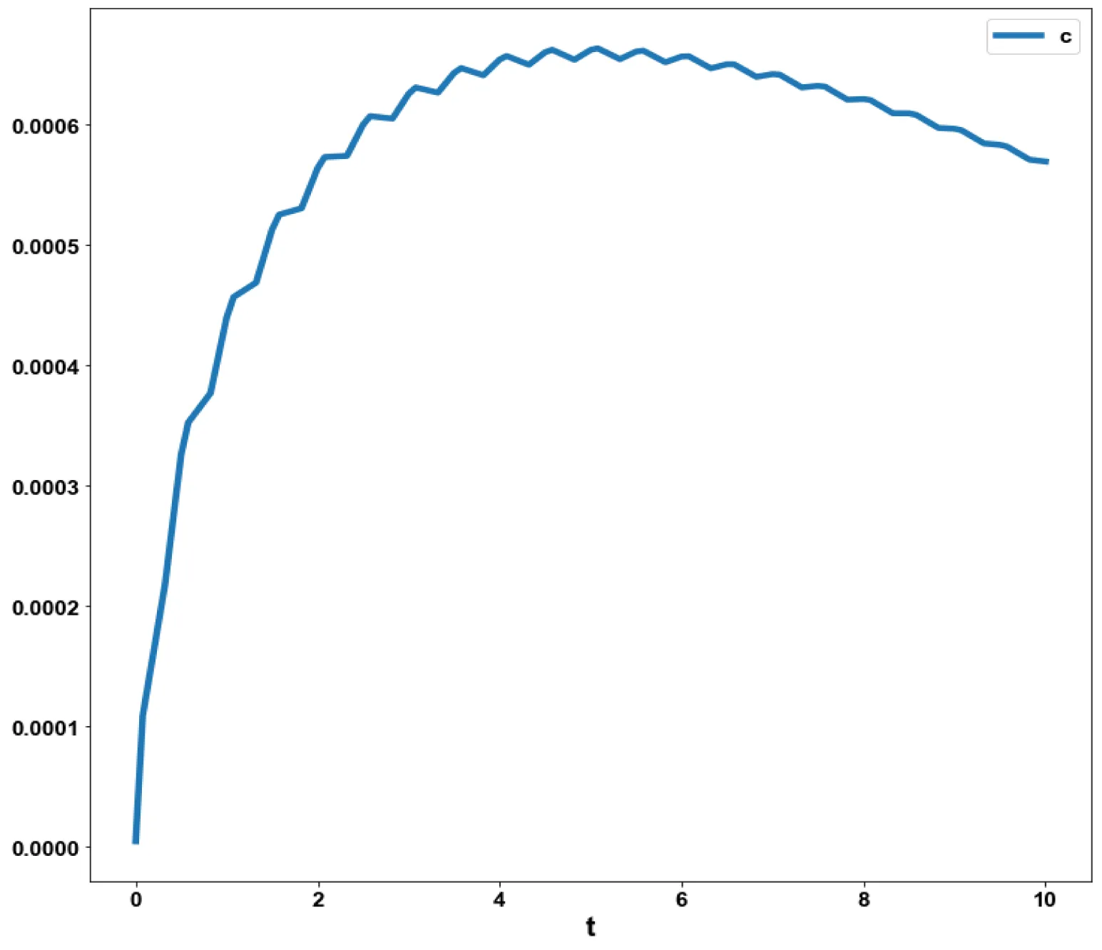
The variables, a and c, which are the concentrations of Aβ and the intracellular Ca2+were minimized. ${\displaystyle \sum _{t_{i=0}}^{t_i=t_f}a(t_i)},{\displaystyle \sum _{t_{i=0}}^{t_i=t_f}b(t_i)},$ was minimized individually and each of them led to a value of ${({\displaystyle \sum _{t_{i=0}}^{t_i=t_f}a(t_i)}-0)}^2+{({\displaystyle \sum _{t_{i=0}}^{t_i=t_f}b(t_i)}-0)}^2$ . The overall optimal control problem will involve the minimization of was minimized subject to the equations governing the model. This led to a value of zero (the Utopia solution.

The various concentration profiles for this MNLMPC calculation are shown in figures 1b-d.

Figure 1a: Biurcation analysis model 1 v1 is bifurcation parameter.

Figure 1b: Biurcation analysis model 1 v2 is bifurcation parameter.

Figure 1c: MNLMPC model a vs t.

Figure 1d: MNLMPC model 1 c vs t.

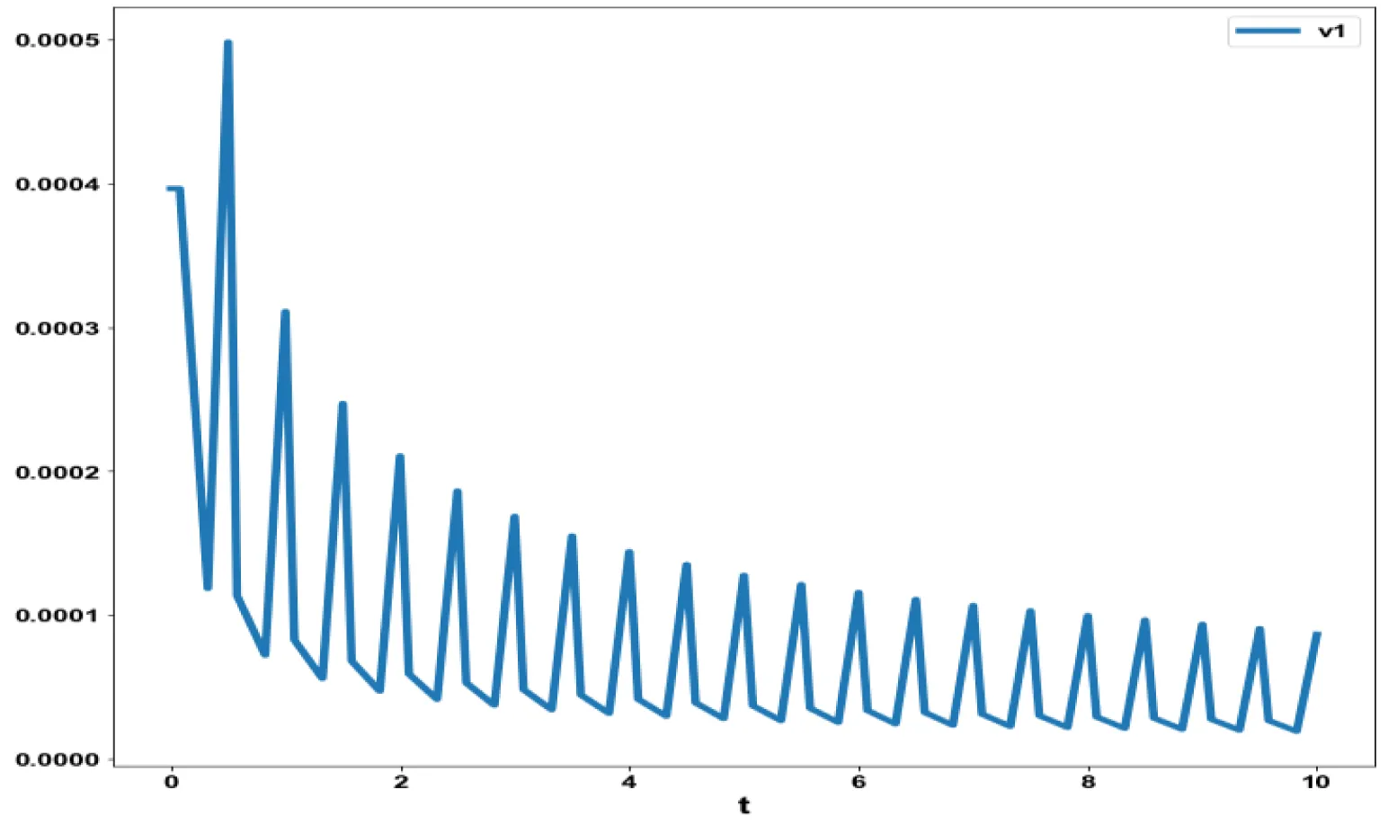
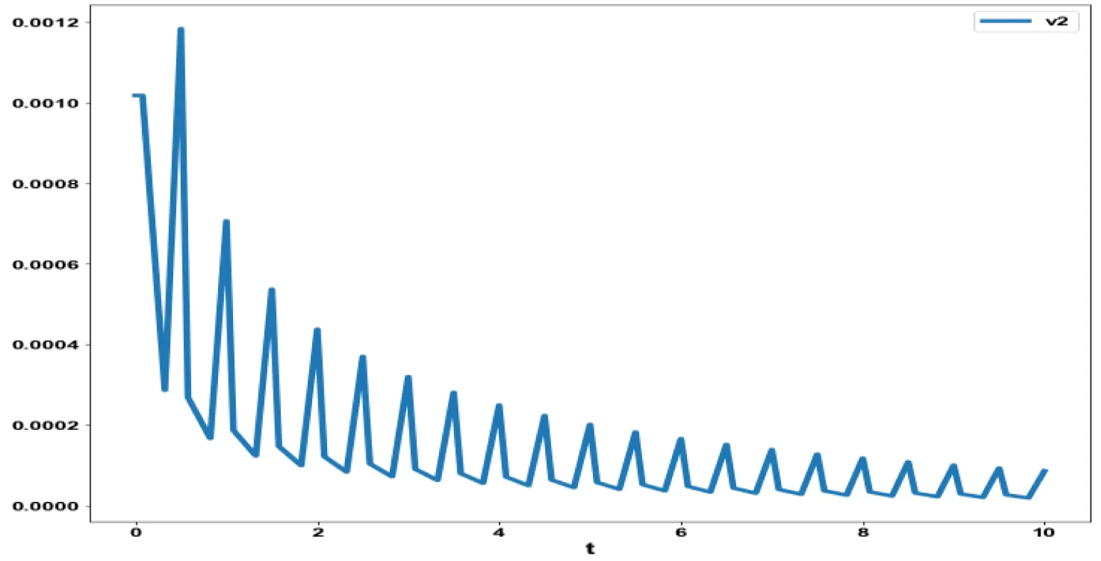
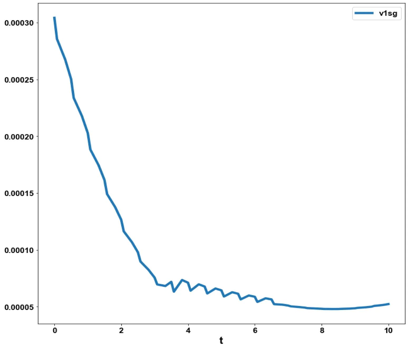
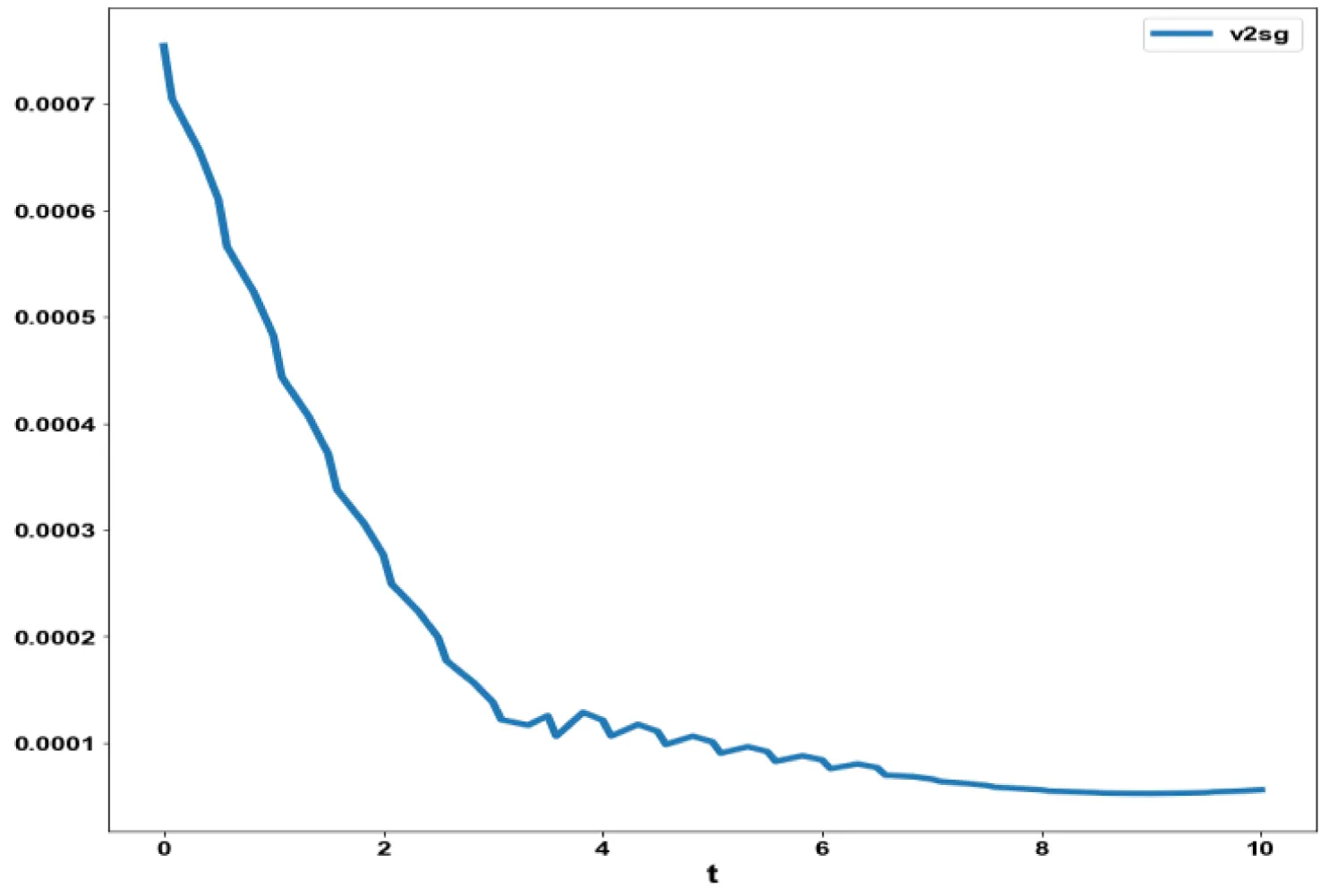
The obtained control profile of s exhibited noise (Figures 1e,f). This was remedied using the Savitzky-Golay Filter. The smoothed-out version of this profile is shown in figures 1g,h. The MNLMPC control values obtained for v1 and v2 are 0.00039 v2 0.001017.

Figure 1e: MNLMPC model 1 v1 vs t.

Figure 1f: MNLMPC model 1 v2 vs t.

Figure 1g: MNLMPC model 1 v1 (Savitzky Golay) vs t.

Figure 1h: MNLMPC model 1 v2 (Savitzky Golay) vs t.

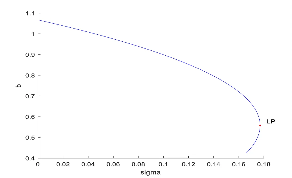
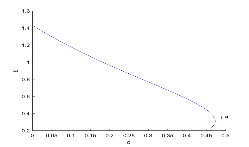
Bifurcation analysis for model 2 revealed the existence of limit points for both the bifurcation parameters sigma and d.

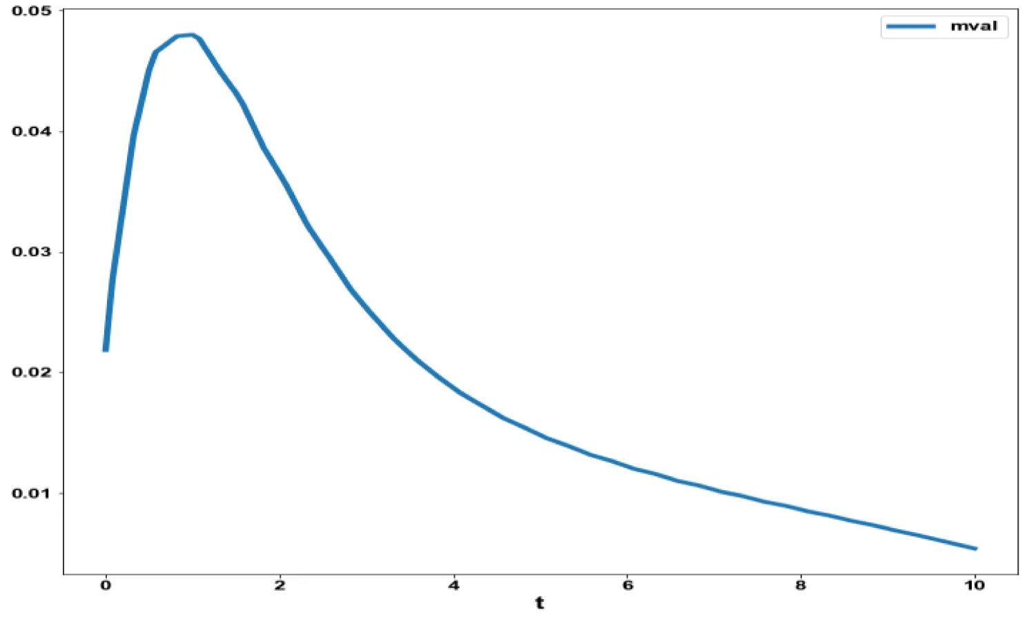
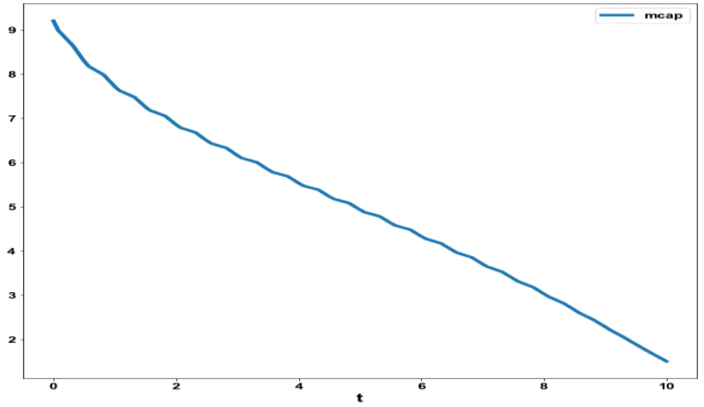
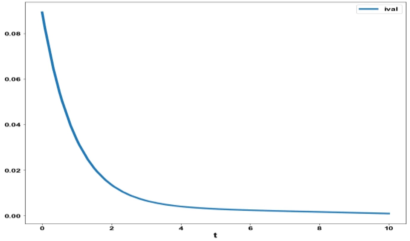
The coordinates for the 2 limit points are (b, bp, mval, mcap, ival, sigma) = (0.557430, 0.929049, 0.527934, 0.499842, 0.178902, 0.177014) and (b, bp, mval, mcap, ival, d) = (0.310730, 0.517884, 0.394164, 0.991528, 0.235058, 0.473347). These limit points are shown in figures 2a,b. The limit points cause the profiles to change direction and this is shown in the figures.

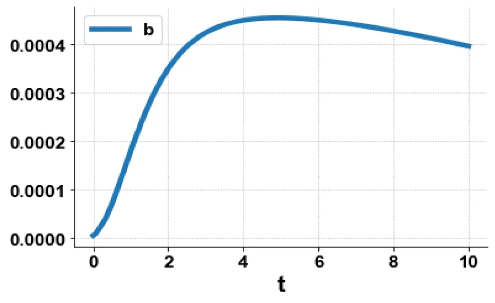
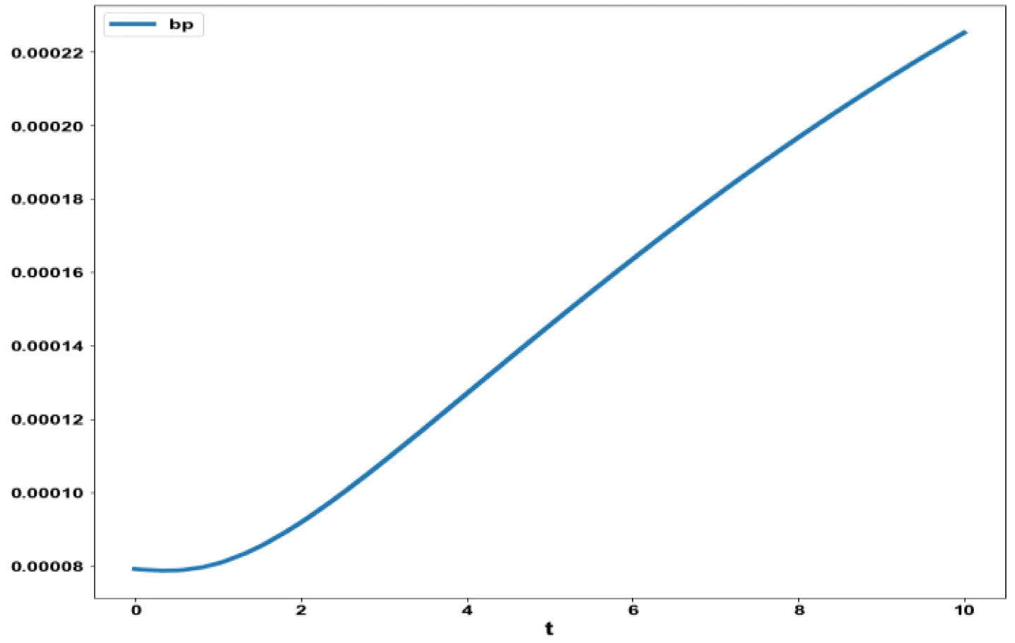
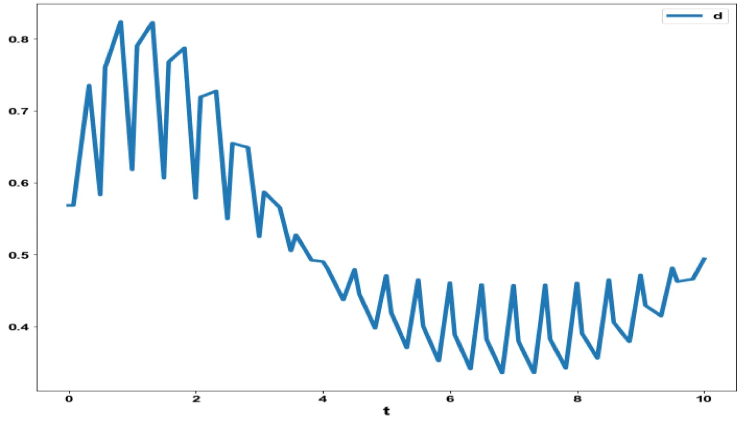
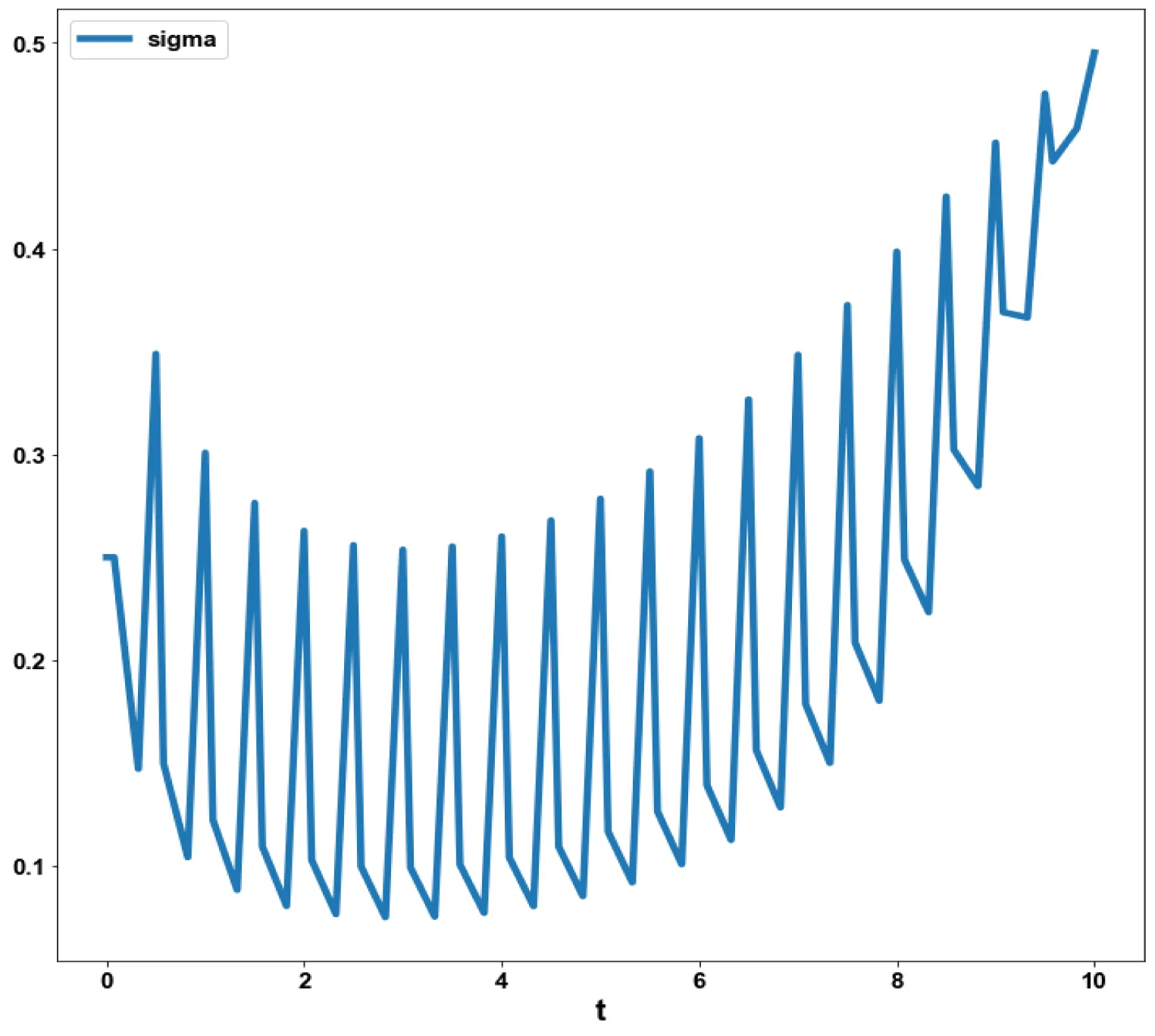
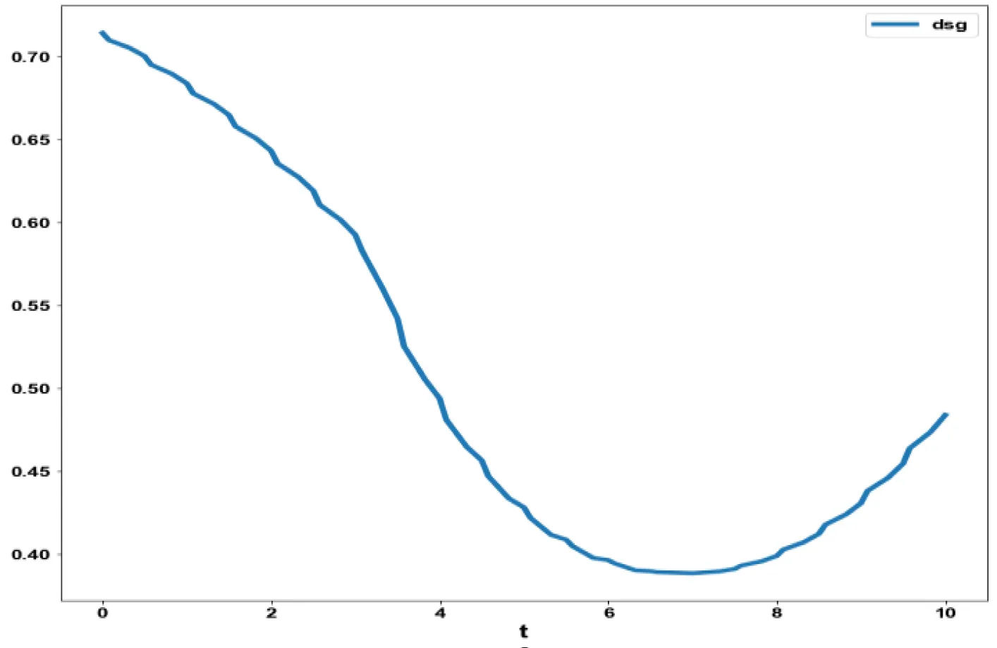
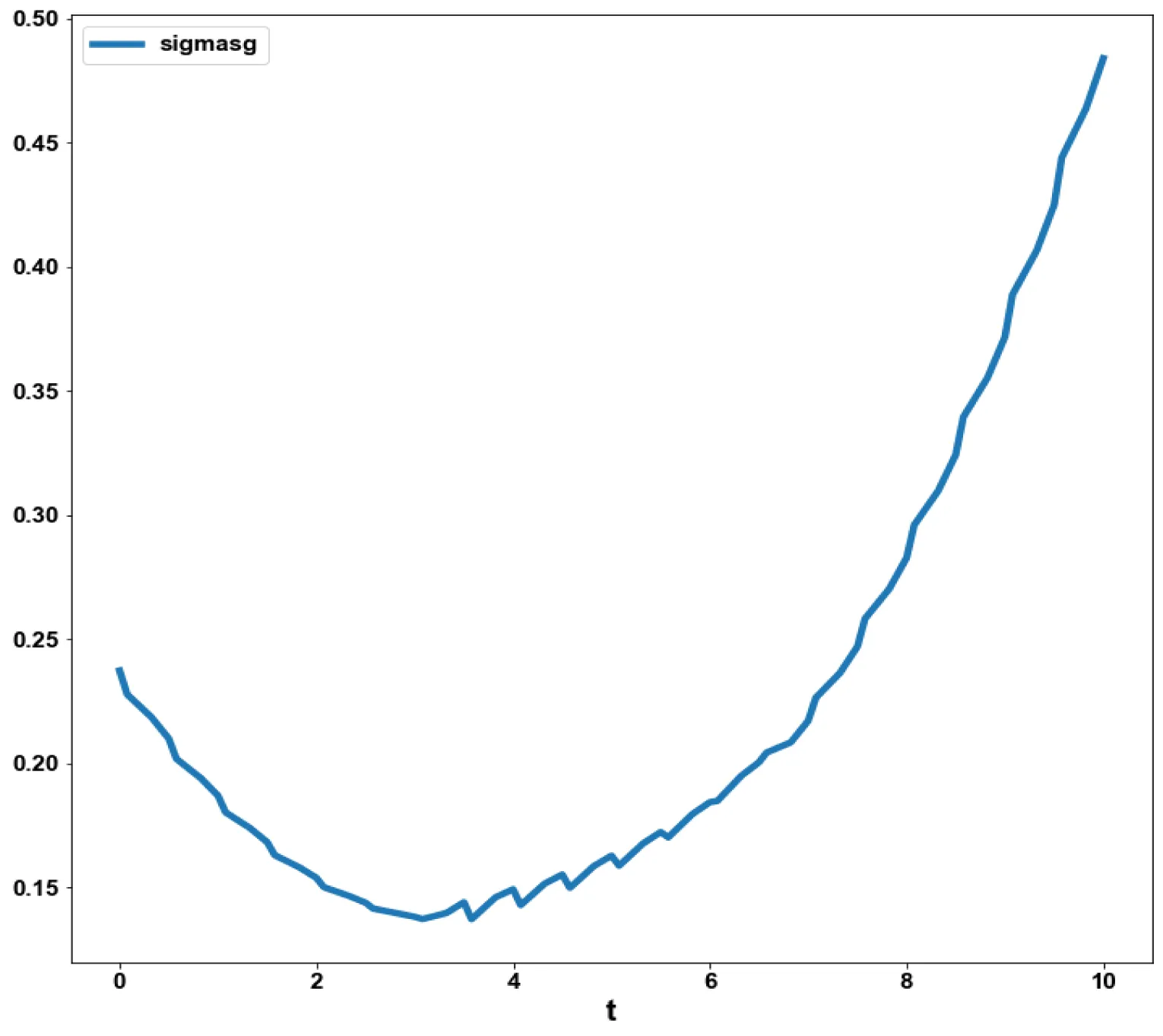
The variables b and bp which are the oligomer concentration and the concentration of oligomers in plaques were minimized. was minimized individually and each of them led to a value of 0 . The overall optimal control problem will involve the minimization of was minimized subject to the equations governing the model. This led to a value of zero (the Utopia solution. The various concentration profiles for this MNLMPC calculation are shown in figures 2c-g. The obtained control profile of s exhibited noise (Figures 2h,i). This was remedied using the Savitzky-Golay Filter. The smoothed-out version of this profile is shown in figures 2j,k. The MNLMPC control values obtained for sigma and d are 0.2499 and 0.5683.

Figure 2a: Bifurcation diagram model 2 sigma is bifurcation parameter.

Figure 2b: Bifurcation diagram model 2 d is bifurcation parameter.

Figure 2c: MNLMPC model 2 b vs t.

Figure 2d: MNLMPC model 2 bp vs t.

Figure 2e: MNLMPC model mval vs t.

Figure 2f: MNLMPC model mcap vs t.

Figure 2g: MNLMPC model ival vs t.

Figure 2h: MNLMPC model d vs t.

Figure 2i: MNLMPC model 2 sigma vs t.

Figure 2j: MNLMPC d (Savitzky Golay) vs t.

Figure 2k: MNLMPC model 2 sigma (Savitzky Golay) vs t.

In both the cases, the MNLMPC calculations converged to the Utopia solution, validating the analysis of Sridhar LN. [66], which showed that the presence of a limit point enables the MNLMPC calculations to reach the best possible (Utopia) solution. The limit points cause a change in the direction of the profiles, and this singularity creates a turning point which enables the MNLMPC to converge to the Utopia solution.

Bifurcation analysis and multiobjective nonlinear model predictive control calculations were performed on two Alzheimer's disease models. The bifurcation analysis revealed the existence of limit points. The limit points (which produced multiple steady-state solutions originating from a singular point) are very beneficial as they caused the multiojective nonlinear model predictive calculations to converge to the Utopia point (the best possible solution) in both models. A combination of bifurcation analysis and multiobjective nonlinear model predictive control for Alzheimer's disease models is the main contribution of this paper.

All data used is presented in the paper

The author, Dr. Lakshmi N Sridhar has no conflict of interest.

Dr. Sridhar thanks Dr. Carlos Ramirez and Dr. Suleiman for encouraging him to write single-author papers.

1. Chao CC, Hu S, Frey WH 2nd, Ala TA, Tourtellotte WW, Peterson PK. Transforming growth factor beta in Alzheimer's disease. Clin Diagn Lab Immunol. 1994 Jan;1(1):109-10. doi: 10.1128/cdli.1.1.109-110.1994. PMID: 7496909; PMCID: PMC368205.
2. Lue LF, Kuo YM, Roher AE, Brachova L, Shen Y, Sue L, Beach T, Kurth JH, Rydel RE, Rogers J. Soluble amyloid beta peptide concentration as a predictor of synaptic change in Alzheimer's disease. Am J Pathol. 1999 Sep;155(3):853-62. doi: 10.1016/s0002-9440(10)65184-x. PMID: 10487842; PMCID: PMC1866907.
3. Mehta PD, Pirttilä T, Mehta SP, Sersen EA, Aisen PS, Wisniewski HM. Plasma and cerebrospinal fluid levels of amyloid beta proteins 1-40 and 1-42 in Alzheimer disease. Arch Neurol. 2000 Jan;57(1):100-5. doi: 10.1001/archneur.57.1.100. PMID: 10634455.
4. Penkowa M, Giralt M, Carrasco J, Hadberg H, Hidalgo J. Impaired inflammatory response and increased oxidative stress and neurodegeneration after brain injury in interleukin-6-deficient mice. Glia. 2000 Dec;32(3):271-85. doi: 10.1002/1098-1136(200012)32:3<271::aid-glia70>3.0.co;2-5. PMID: 11102968.
5. Penkowa M, Molinero A, Carrasco J, Hidalgo J. Interleukin-6 deficiency reduces the brain inflammatory response and increases oxidative stress and neurodegeneration after kainic acid-induced seizures. Neuroscience. 2001;102(4):805-18. doi: 10.1016/s0306-4522(00)00515-7. PMID: 11182244.
6. Wyss-Coray T, Lin C, Yan F, Yu GQ, Rohde M, McConlogue L, Masliah E, Mucke L. TGF-beta1 promotes microglial amyloid-beta clearance and reduces plaque burden in transgenic mice. Nat Med. 2001 May;7(5):612-8. doi: 10.1038/87945. PMID: 11329064.
7. Jacobsen JS, Wu CC, Redwine JM, Comery TA, Arias R, Bowlby M, Martone R, Morrison JH, Pangalos MN, Reinhart PH, Bloom FE. Early-onset behavioral and synaptic deficits in a mouse model of Alzheimer's disease. Proc Natl Acad Sci U S A. 2006 Mar 28;103(13):5161-6. doi: 10.1073/pnas.0600948103. Epub 2006 Mar 20. PMID: 16549764; PMCID: PMC1405622.
8. Wyss-Coray T. Tgf-Beta pathway as a potential target in neurodegeneration and Alzheimer's. Curr Alzheimer Res. 2006 Jul;3(3):191-5. doi: 10.2174/156720506777632916. PMID: 16842094.
9. Das P, Golde T, et al. Dysfunction of TGF-β signaling in Alzheimer’s disease. The Journal of clinical investigation. 2006;116(11):2855-7 Das P, Golde T. Dysfunction of TGF-beta signaling in Alzheimer's disease. J Clin Invest. 2006 Nov;116(11):2855-7. doi: 10.1172/JCI30284. PMID: 17080189; PMCID: PMC1626134.
10. Tobinick E, Gross H, Weinberger A, Cohen H. TNF-alpha modulation for treatment of Alzheimer's disease: a 6-month pilot study. MedGenMed. 2006 Apr 26;8(2):25. PMID: 16926764; PMCID: PMC1785182.
11. Green KN, Smith IF, Laferla FM. Role of calcium in the pathogenesis of Alzheimer's disease and transgenic models. Subcell Biochem. 2007;45:507-21. doi: 10.1007/978-1-4020-6191-2_19. PMID: 18193650.
12. ADAPT Research Group; Lyketsos CG, Breitner JC, Green RC, Martin BK, Meinert C, Piantadosi S, Sabbagh M. Naproxen and celecoxib do not prevent AD in early results from a randomized controlled trial. Neurology. 2007 May 22;68(21):1800-8. doi: 10.1212/01.wnl.0000260269.93245.d2. Epub 2007 Apr 25. PMID: 17460158.
13. Town T, Laouar Y, Pittenger C, Mori T, Szekely CA, Tan J, Duman RS, Flavell RA. Blocking TGF-beta-Smad2/3 innate immune signaling mitigates Alzheimer-like pathology. Nat Med. 2008 Jun;14(6):681-7. doi: 10.1038/nm1781. Epub 2008 Jun 1. PMID: 18516051; PMCID: PMC2649699.
14. Cheung KH, Shineman D, Müller M, Cárdenas C, Mei L, Yang J, Tomita T, Iwatsubo T, Lee VM, Foskett JK. Mechanism of Ca2+ disruption in Alzheimer's disease by presenilin regulation of InsP3 receptor channel gating. Neuron. 2008 Jun 26;58(6):871-83. doi: 10.1016/j.neuron.2008.04.015. PMID: 18579078; PMCID: PMC2495086.
15. Bezprozvanny I, Mattson MP. Neuronal calcium mishandling and the pathogenesis of Alzheimer's disease. Trends Neurosci. 2008 Sep;31(9):454-63. doi: 10.1016/j.tins.2008.06.005. Epub 2008 Jul 31. PMID: 18675468; PMCID: PMC2566585.
16. Bojarski L, Herms J, Kuznicki J. Calcium dysregulation in Alzheimer's disease. Neurochem Int. 2008 Mar-Apr;52(4-5):621-33. doi: 10.1016/j.neuint.2007.10.002. Epub 2007 Oct 5. PMID: 18035450.
17. ADAPT Research Group; Martin BK, Szekely C, Brandt J, Piantadosi S, Breitner JC, Craft S, Evans D, Green R, Mullan M. Cognitive function over time in the Alzheimer's Disease Anti-inflammatory Prevention Trial (ADAPT): results of a randomized, controlled trial of naproxen and celecoxib. Arch Neurol. 2008 Jul;65(7):896-905. doi: 10.1001/archneur.2008.65.7.nct70006. Epub 2008 May 12. PMID: 18474729; PMCID: PMC2925195.
18. Lopez JR, Lyckman A, Oddo S, Laferla FM, Querfurth HW, Shtifman A. Increased intraneuronal resting [Ca2+] in adult Alzheimer's disease mice. J Neurochem. 2008 Apr;105(1):262-71. doi: 10.1111/j.1471-4159.2007.05135.x. Epub 2007 Nov 16. PMID: 18021291.
19. Nelson O, Supnet C, Liu H, Bezprozvanny I. Familial Alzheimer's disease mutations in presenilins: effects on endoplasmic reticulum calcium homeostasis and correlation with clinical phenotypes. J Alzheimers Dis. 2010;21(3):781-93. doi: 10.3233/JAD-2010-100159. PMID: 20634584; PMCID: PMC4996666.
20. Puri IK, Li L. Mathematical modeling for the pathogenesis of Alzheimer's disease. PLoS One. 2010 Dec 14;5(12):e15176. doi: 10.1371/journal.pone.0015176. PMID: 21179474; PMCID: PMC3001872.
21. Berridge MJ. Calcium hypothesis of Alzheimer's disease. Pflugers Arch. 2010 Feb;459(3):441-9. doi: 10.1007/s00424-009-0736-1. Epub 2009 Oct 1. PMID: 19795132.
22. Imbimbo BP, Solfrizzi V, Panza F. Are NSAIDs useful to treat Alzheimer's disease or mild cognitive impairment? Front Aging Neurosci. 2010 May 21;2:19. doi: 10.3389/fnagi.2010.00019. PMID: 20725517; PMCID: PMC2912027.
23. Berridge MJ. Calcium signalling and Alzheimer's disease. Neurochem Res. 2011 Jul;36(7):1149-56. doi: 10.1007/s11064-010-0371-4. Epub 2010 Dec 24. PMID: 21184278.
24. Anastasio TJ. Data-driven modeling of Alzheimer disease pathogenesis. J Theor Biol. 2011 Dec 7;290:60-72. doi: 10.1016/j.jtbi.2011.08.038. Epub 2011 Sep 5. PMID: 21920373.
25. Camandola S, Mattson MP. Aberrant subcellular neuronal calcium regulation in aging and Alzheimer's disease. Biochim Biophys Acta. 2011 May;1813(5):965-73. doi: 10.1016/j.bbamcr.2010.10.005. Epub 2010 Oct 13. PMID: 20950656; PMCID: PMC3032815.
26. Ho M, Hoke DE, Chua YJ, Li QX, Culvenor JG, Masters C, White AR, Evin G. Effect of Metal Chelators on γ-Secretase Indicates That Calcium and Magnesium Ions Facilitate Cleavage of Alzheimer Amyloid Precursor Substrate. Int J Alzheimers Dis. 2010 Dec 28;2011:950932. doi: 10.4061/2011/950932. PMID: 21253550; PMCID: PMC3021864.
27. Itkin A, Dupres V, Dufrêne YF, Bechinger B, Ruysschaert JM, Raussens V. Calcium ions promote formation of amyloid β-peptide (1-40) oligomers causally implicated in neuronal toxicity of Alzheimer's disease. PLoS One. 2011 Mar 28;6(3):e18250. doi: 10.1371/journal.pone.0018250. PMID: 21464905; PMCID: PMC3065491.
28. Müller M, Cárdenas C, Mei L, Cheung KH, Foskett JK. Constitutive cAMP response element binding protein (CREB) activation by Alzheimer's disease presenilin-driven inositol trisphosphate receptor (InsP3R) Ca2+ signaling. Proc Natl Acad Sci U S A. 2011 Aug 9;108(32):13293-8. doi: 10.1073/pnas.1109297108. Epub 2011 Jul 22. PMID: 21784978; PMCID: PMC3156223.
29. Schmidt V, Baum K, Lao A, Rateitschak K, Schmitz Y, Teichmann A, Wiesner B, Petersen CM, Nykjaer A, Wolf J, Wolkenhauer O, Willnow TE. Quantitative modelling of amyloidogenic processing and its influence by SORLA in Alzheimer's disease. EMBO J. 2012 Jan 4;31(1):187-200. doi: 10.1038/emboj.2011.352. Epub 2011 Oct 11. PMID: 21989385; PMCID: PMC3252570.
30. Ma T, Gong K, Yan Y, Song B, Zhang X, Gong Y. Mitochondrial modulation of store-operated Ca(2+) entry in model cells of Alzheimer's disease. Biochem Biophys Res Commun. 2012 Sep 21;426(2):196-202. doi: 10.1016/j.bbrc.2012.08.062. Epub 2012 Aug 23. PMID: 22935417.
31. Woods NK, Padmanabhan J. Neuronal calcium signaling and Alzheimer's disease. Adv Exp Med Biol. 2012;740:1193-217. doi: 10.1007/978-94-007-2888-2_54. PMID: 22453989.
32. De Kimpe L, Bennis A, Zwart R, van Haastert ES, Hoozemans JJ, Scheper W. Disturbed Ca2+ homeostasis increases glutaminyl cyclase expression; connecting two early pathogenic events in Alzheimer's disease in vitro. PLoS One. 2012;7(9):e44674. doi: 10.1371/journal.pone.0044674. Epub 2012 Sep 7. PMID: 22970285; PMCID: PMC3436868.
33. Berridge MJ. Dysregulation of neural calcium signaling in Alzheimer disease, bipolar disorder and schizophrenia. Prion. 2013 Jan-Feb;7(1):2-13. doi: 10.4161/pri.21767. Epub 2012 Aug 16. PMID: 22895098; PMCID: PMC3609045.
34. Lopategui Cabezas I, Herrera Batista A, Pentón Rol G. The role of glial cells in Alzheimer disease: potential therapeutic implications. Neurologia. 2014 Jun;29(5):305-9. English, Spanish. doi: 10.1016/j.nrl.2012.10.006. Epub 2012 Dec 14. PMID: 23246214.
35. Chen JH, Ke KF, Lu JH, Qiu YH, Peng YP. Protection of TGF-β1 against neuroinflammation and neurodegeneration in Aβ1-42-induced Alzheimer's disease model rats. PLoS One. 2015 Feb 6;10(2):e0116549. doi: 10.1371/journal.pone.0116549. PMID: 25658940; PMCID: PMC4319949.
36. von Bernhardi R, Cornejo F, Parada GE, Eugenín J. Role of TGFβ signaling in the pathogenesis of Alzheimer's disease. Front Cell Neurosci. 2015 Oct 28;9:426. doi: 10.3389/fncel.2015.00426. PMID: 26578886; PMCID: PMC4623426.
37. Bertsch M, Franchi B, Marcello N, Tesi MC, Tosin A. Alzheimer's disease: a mathematical model for onset and progression. Math Med Biol. 2017 Jun 1;34(2):193-214. doi: 10.1093/imammb/dqw003. PMID: 27079222.
38. Hao W, Friedman A. Mathematical model on Alzheimer’s disease. BMC systems biology. 2016;10(1):1-18. doi: 10.1186/s12918-016-0348-2.
39. Forloni G, Balducci C. Alzheimer's Disease, Oligomers, and Inflammation. J Alzheimers Dis. 2018;62(3):1261-1276. doi: 10.3233/JAD-170819. PMID: 29562537; PMCID: PMC5869993.
40. Kinney JW, Bemiller SM, Murtishaw AS, Leisgang AM, Salazar AM, Lamb BT. Inflammation as a central mechanism in Alzheimer's disease. Alzheimers Dement (N Y). 2018 Sep 6;4:575-590. doi: 10.1016/j.trci.2018.06.014. PMID: 30406177; PMCID: PMC6214864.
41. Zhu M, Wang X, Sun L, Schultzberg M, Hjorth E. Can inflammation be resolved in Alzheimer's disease? Ther Adv Neurol Disord. 2018 Aug 9;11:1756286418791107. doi: 10.1177/1756286418791107. PMID: 30116300; PMCID: PMC6088473.
42. Ozben T, Ozben S. Neuro-inflammation and anti-inflammatory treatment options for Alzheimer's disease. Clin Biochem. 2019 Oct;72:87-89. doi: 10.1016/j.clinbiochem.2019.04.001. Epub 2019 Apr 4. PMID: 30954437.
43. Ali MM, Ghouri RG, Ans AH, Akbar A, Toheed A. Recommendations for Anti-inflammatory Treatments in Alzheimer's Disease: A Comprehensive Review of the Literature. Cureus. 2019 May 8;11(5):e4620. doi: 10.7759/cureus.4620. PMID: 31312547; PMCID: PMC6615583.
44. Ciuperca IS, Dumont M, Lakmeche A, Mazzocco P, Pujo-Menjouet L, Rezaei H, Léon MT. Alzheimer's disease and prion: An in vitro mathematical model. Discrete & Continuous Dynamical Systems-B. 2019;24(10):5225-5260. doi: 10.3934/dcdsb.2019057.
45. Andrade-Restrepo M, Lemarre P, Pujo-Menjouet L, Tine LM, Ciuperca SI. Modeling the spatial propagation of Aβ oligomers in Alzheimer’s Disease. ESAIM: Proceedings and Surveys. 2020;67:30-45. doi: 10.1051/proc/202067003.
46. Rivers-Auty J, Mather AE, Peters R, Lawrence CB, Brough D. Anti-inflammatories in Alzheimer's disease-potential therapy or spurious correlate? Brain Commun. 2020 Jul 24;2(2):fcaa109. doi: 10.1093/braincomms/fcaa109. PMID: 33134914; PMCID: PMC7585697.
47. Huang LK, Chao SP, Hu CJ. Clinical trials of new drugs for Alzheimer disease. J Biomed Sci. 2020 Jan 6;27(1):18. doi: 10.1186/s12929-019-0609-7. PMID: 31906949; PMCID: PMC6943903.
48. Li H, Zhao H. Mathematical model of Alzheimer’s disease with prion proteins interactions and treatment. Applied Mathematics and Computation. 2022;433(15):127377. doi: 10.1016/j.amc.2022.127377.
49. Hu J, Zhang Q, Meyer-Baese A, Ye M. Finite-time stability and optimal control of a stochastic reaction diffusion model for Alzheimer’s disease with impulse and time-varying delay. Applied Mathematical Modelling. 2022;102:511-39.  doi: 10.1016/j.apm.2021.10.004.
50. Hao W, Lenhart S, Petrella JR. Optimal anti-amyloid-beta therapy for Alzheimer's disease via a personalized mathematical model. PLoS Comput Biol. 2022 Sep 2;18(9):e1010481. doi: 10.1371/journal.pcbi.1010481. PMID: 36054214; PMCID: PMC9477429.
51. Al-Ghraiybah NF, Wang J, Alkhalifa AE, Roberts AB, Raj R, Yang E, Kaddoumi A. Glial Cell-Mediated Neuroinflammation in Alzheimer's Disease. Int J Mol Sci. 2022 Sep 12;23(18):10572. doi: 10.3390/ijms231810572. PMID: 36142483; PMCID: PMC9502483.
52. Pal S, Melnik R. Modelling of anti-amyloid-beta therapy for alzheimer’s disease. In: International Work-Conference on Bioinformatics and Biomedical Engineering. 2023;431-42.
53. van Dyck CH, Swanson CJ, Aisen P, Bateman RJ, Chen C, Gee M, Kanekiyo M, Li D, Reyderman L, Cohen S, Froelich L, Katayama S, Sabbagh M, Vellas B, Watson D, Dhadda S, Irizarry M, Kramer LD, Iwatsubo T. Lecanemab in Early Alzheimer's Disease. N Engl J Med. 2023 Jan 5;388(1):9-21. doi: 10.1056/NEJMoa2212948. Epub 2022 Nov 29. PMID: 36449413.
54. Ciuperca I, Pujo-Menjouet L, Matar-Tine L, Torres N, Volpert V. A qualitative analysis of an Aβ-monomer model with inflammation processes for Alzheimer's disease. R Soc Open Sci. 2024 May 15;11(5):231536. doi: 10.1098/rsos.231536. PMID: 39076807; PMCID: PMC11285901.
55. De Caluwé J, Dupont G. The progression towards Alzheimer's disease described as a bistable switch arising from the positive loop between amyloids and Ca(2+). J Theor Biol. 2013 Aug 21;331:12-8. doi: 10.1016/j.jtbi.2013.04.015. Epub 2013 Apr 21. PMID: 23614875.
56. Torres N, Molina E, Pujo-Menjouet L. An optimal control problem for anti-inflammatory treatments of Alzheimer's disease. J Math Biol. 2025 May 26;91(1):1. doi: 10.1007/s00285-025-02227-8. PMID: 40418238.
57. Dhooge A, Govearts W, Kuznetsov, AY. MATCONT: A Matlab package for numerical bifurcation analysis of ODEs,   ACM transactions on Mathematical software. 2023;29(2):141-164. doi: 10.1145/779359.77936.
58. Dhooge A, Govaerts W, Kuznetsov YA, Mestrom W, Riet AM. Cl_matcont; a continuation toolbox in matlab. SAC '03: Proceedings of the 2003 ACM symposium on Applied computing.2004;161-166. doi: 10.1145/952532.952567.
59. Kuznetsov YA. Elements of applied bifurcation theory. Springer Nature. 1998.
60. Kuznetsov YA. Five lectures on numerical bifurcation analysis. Utrecht University,NL. 2009.
61. Govaerts WJF. Numerical methods for bifurcations of dynamical equilibria. Society for Industrial and Applied Mathematics. 2000. doi: 10.1137/1.9780898719543.
62. Flores TA, Pilar Morales, Martin RT. Multiobjective nonlinear model predictive control of a class of chemical reactors . Industrial & Engineering Chemistry Research. 2012;51(17):5891-5899. doi: 10.1021/ie201742e.
63. Hart WE, Carl DL, Jean PW, David LW, Gabriel AH, Bethany LN, John DS. Pyomo – Optimization modeling in python. 2nd ed. Springer Nature; 2017.
64. Wächter A, Biegler L. On the implementation of an interior-point filter line-search algorithm for large-scale nonlinear programming. Mathematical Programming. 2005;106:25-57 . doi: 10.1007/s10107-004-0559-y.
65. Tawarmalani M, Sahinidis NV. A polyhedral branch-and-cut approach to global optimization. Mathematical Programming. 2005;103(2):225-249. doi: 10.1007/s10107-005-0581-8.
66. Sridhar LN. Coupling bifurcation analysis and multiobjective nonlinear model predictive control. Austin Chemical Engineering. 2024;10(3):1107.
67. Upreti SR. Optimal control for chemical engineers. 1st ed. Taylor and Francis; 2013.