> Environmental Sciences. 2021 September 30;2(9):865-869. doi: 10.37871/jbres1325.
Modeling of the Number of Cold Fronts in Cuba Using the Objective Regressive Regression (ROR) Methodology; Impact of Sunspots
Ricardo Oses Rodriguez1*, Rigoberto Fimia Duarte2 and Alfredo Gonzalez Meneses3
2Faculty of Health Technology, University of Medical Sciences, Villa Clara, Cuba
3Construtora Company of the Electricity Industry of Villa Clara (ECIE), Cuba
Abstract
The objective of this work is to model the variable number of cold fronts that affect the Cuban territory in a winter season for a long series of data, to establish if the trend is significant and to see which are the main statistics of the model, to observe the impact of prediction using the number of sunspots with the help of Objective Regressive ROR modeling. In this work, the series of cold fronts per season that affect the Cuban territory was modeled in the years from the 1916-1917 seasons to the 2006-2007 seasons. There are more moderate cold fronts than any other front, on average there are more classic fronts than any other type, on average 19 fronts can be presented per season with a standard deviation of 4.8 Sunspots and they only have a significant linear correlation with sunspots. In moderate fronts, as the stains increase, the number of fronts decreases. The ROR model explains 98% of the variance with an error of 4.2 cases and depends on the fronts returned in 5 seasons, which could coincide with the ENSO event, and also depends on the number of sunspots returned in 12 years. From 1916-1917 approximately the 1952-1953 season, moderate fronts predominated, later from 1953-1954 to the end of the data, weak fronts predominate over the rest with some exceptions throughout history. No significant trend was observed in the model. It is concluded that forecasts of the number of cold fronts can be made with the variable number of sunspots.
Introduction
The ability to predict climate variables in advance offers the possibility of being able to act in time and reduce adverse impacts, that is, to adapt to the effects of climate change and variability. Increased preparedness for extreme weather events contributes significantly to reducing vulnerability [1].
The climate prediction is one that foresees the average weather conditions for periods of duration from one month to one or two years. In practice, two large groups are distinguished: those who make forecasts of the value of the element in question, deterministic forecasts, and those who predict the probability of occurrence of a certain value of the element, probabilistic forecasts, and this work uses deterministic statistical models using the regressive objective regression.
In the most recent Scientific Assessment report of the Intergovernmental Panel of Experts on Climate Change (IPCC, 2007a) [2], it is concluded that warming is unequivocal, this will bring disruptions in other climatic variables such as precipitation or rainfall and also in behavior of the winds and in the behavior of the cold fronts.
Forecasts of both the weather and climate are an important element in the life of modern society. Having a forecasting system on several scales (monthly, daily and annual) allows us to have a powerful tool in the planning of economic and social activities.
In Cuba, important work has been carried out to determine between groups of primary and calculated predictors of a dynamic type and of the Temperature-Humidity complex the potential future predictors that intervene in the selection of the real predictors for the rain forecast in Cuba [3]. In the present work, a pure statistical forecast is used, looking in previous steps (Lags) for the in formativeness of the process to be modeled, either the number of fronts that affect Cuba as well as the sunspots that are measured globally.
Sunspots are a factor that influences the behavior of cold fronts at least in short periods, however other authors have indicated that according to satellite measurements that sunrise and its variability has contributed significantly to the increase in global average temperature in the last 50 years [4-8].
Locally, however, the correlations between solar activity and mean time may be due more than to the global trend; this has been discussed for the cases of the El Niño-Southern Oscillation event even in the present 9.
Solar irradiation and the flow of the sun’s eruptions directly towards the earth is the main source of its energy. The Sun moves on several scales - from billions of years its luminosity will increase until it becomes a red giant, every 11 years the cycle of sunspots is presented while the flares occur in a matter of minutes, releasing large amounts of energy [9].
The objective of this work is to model the variable number of cold fronts that affect the Cuban territory in a winter season for a long series of data, to establish if the trend is significant and to see which are the main statistics of the model, to observe the impact of predicting using the number of sunspots with the help of Objective Regressive ROR modeling [10,11].
Materials and Methods
In this work, the series of cold fronts per season that affect the Cuban territory was modeled in the years from the 1916-1917 season to the 2006-2007 season, it also had the data on sunspots available to the climate department of the Provincial Meteorological Center of Villa Clara, Cuba.
Results and Discussion
In (Table 1) the main statistics of the 91 seasons of cold fronts that have affected Cuba, as well as the intensities for Weak, Moderate and Strong, also by type of front, Classic, revision or secondary. There are more moderate cold fronts than any other front, on average there are more classic fronts than any other type on average 19 fronts can be presented per season with a standard deviation of 4.8.
| Table 1: Descriptive statistics. | |||||
| N | Minimum | Maximum | Mean | Standard deviation | |
| Weak | 91 | 0 | 21 | 9.03 | 4.825 |
| Moderate | 91 | 2 | 19 | 9.01 | 3.526 |
| Strong | 91 | 0 | 9 | 1.65 | 1.682 |
| Classic | 91 | 5 | 29 | 15.73 | 4.709 |
| Reverse | 91 | 0 | 11 | 3.02 | 2.963 |
| Secondary | 91 | 0 | 8 | .93 | 1.519 |
| Cuba | 91 | 11 | 35 | 19.69 | 4.841 |
| sunspot | 107 | 2.90000 | 190.20000 | 62.5617575 | 46.65805441 |
| Valid N (per list) | 91 | ||||
The Pearson correlations of the sunspots with respect to the other variables were studied, observing that it only has a significant linear correlation with moderate fronts, as the spots increase, the number of front’s decreases in (Table 2).
| Table 2: Correlations. | ||||||
| sunspot | Classic | Reverse | Secondary | |||
| sunspot | Pearson's correlation | 1 | -.099 | .109 | -.058 | |
| Sig. (Bilateral) | .351 | .302 | .587 | |||
| N | 107 | 91 | 91 | 91 | ||
| Weak | Moderate | Strong | sunspot | |||
| sunspot | Pearson's correlation | .194 | -.257* | .076 | 1 | |
| Sig. (Bilateral) | .065 | .014 | .473 | |||
| N | 91 | 91 | 91 | 107 | ||
| **.The correlation is significant at the 0.01 level (2-tailed). *.The correlation is significant at the 0.05 level (2-tailed). |
||||||
Tables 3,4 shows that the ROR model explains 98% of the variance with an error of 4.2 cases, the Durbin Watson statistic is close to 2, so the model is valid and no further information is necessary in the model.
| Table 3: Summary of the modelc,d. | |||||
| Model | R | R squaredb | R squared fitted | Standard error of the estimate | Durbin-Watson |
| 1 | .981a | .962 | .959 | 4.183 | 2.042 |
| a: Predictors: Step61, DI, DS, Lag12Sunspot, Lag5Frentes b: For regression through the origin (the model without interception) R: Square measures the proportion of the variability in the dependent variable on the origin explained by the regression. This cannot be compared to R squared for models that include intercept c: Dependent variable: FRentesCuba d: Linear regression through the origin |
|||||
| The analysis of variance is significant at 100% with a Fisher's F of 374 | |||||
| Table 4: ANOVAa,b. | |||||
| Model | Sum of squares | gl | Quadratic mean | F | Sig. |
| Regression | 32744.370 | 5 | 6548.874 | 374.328 | .000c |
| Residue | 1294.630 | 74 | 17.495 | ||
| Total | 34039.000d | 79 | |||
| a: Dependent variable: FRentesCuba b: Linear regression through the origin c: Predictors: Step61, DI, DS, Lag12Sunspot, Lag5Frentes d: This total sum of squares is not corrected for the constant because the constant is zero for the regression through the origin |
|||||
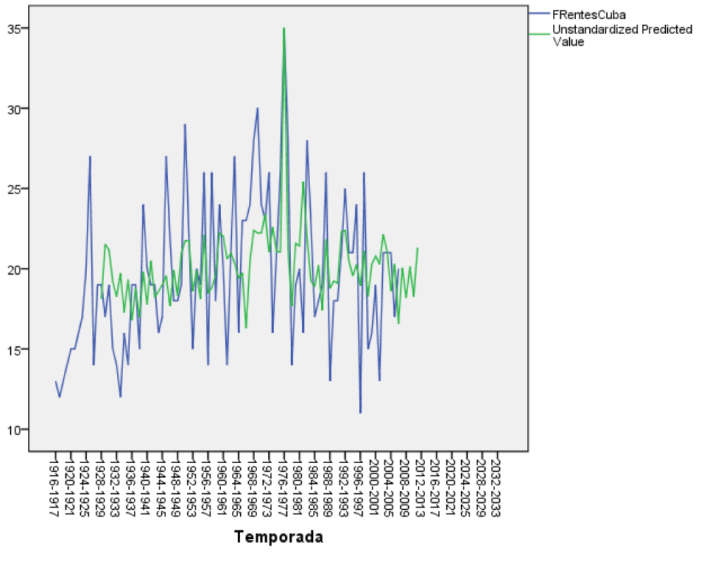
The ROR model (Table 5) of the number of fronts depends on DS and DI, respectively a variable that is formed as a sawtooth and Di as an inverted sawtooth, Lag5Frentes, represents the fronts returned in 5 seasons, which could coincide with the ENSO event, Lag12Sunspot, represents the number of sunspots returned in 12 seasons, which can coincide with the solar cycle which is 11 years, Step 61 corresponds to the 1976-1977 season where a maximum of 35 fronts were presented , which the model estimates as 16. No significant trend was observed in the model.
| Table 5: Coefficientsa,b. | ||||||
| Model | Non-standardized coefficients | Standardized coefficients | t | Sig. | ||
| B | Standard error | Beta | ||||
| 1 | DS | 12.610 | 2.231 | .432 | 5.651 | .000 |
| DI | 14.307 | 2.121 | .484 | 6.745 | .000 | |
| Lag5Frentes | .257 | .099 | .257 | 2.609 | .011 | |
| Lag12Sunspot | .020 | .010 | .081 | 2.066 | .042 | |
| Step61 | 16.267 | 4.281 | .088 | 3.800 | .000 | |
| a: Dependent variable: FRentesCuba | ||||||
| b: Linear regression through the origin | ||||||
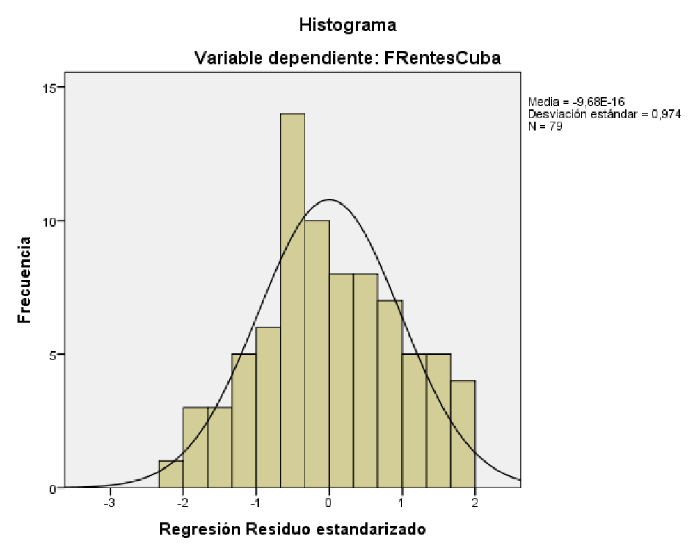
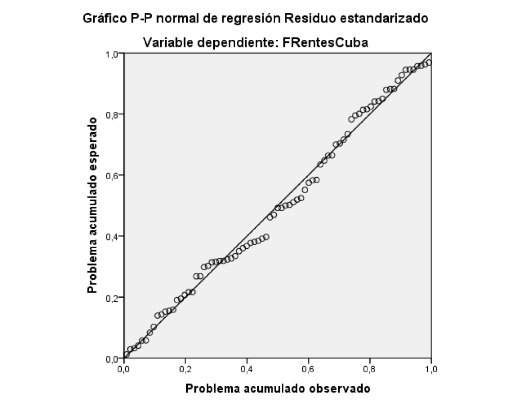
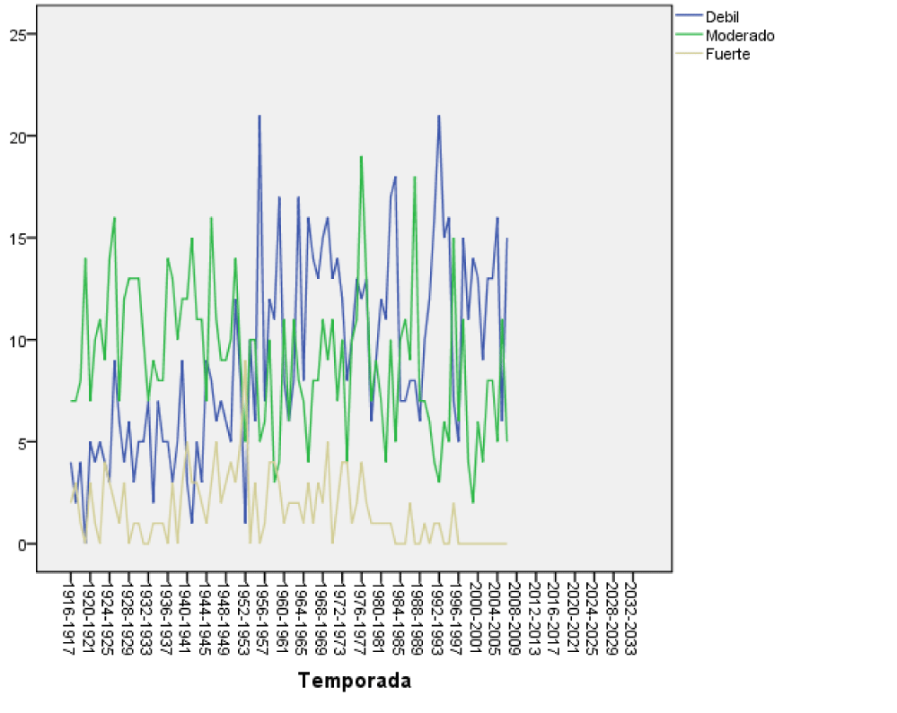
The histogram of the residuals has a zero mean and a deviation close to 1, which is very important for the model (Figure 1). The expected probability of the model against the observed probability presents a straight line, so we are facing a valid model to predict (Figure 2). Finally, in (Figures 3,4) a graph was made of the behavior of the fronts by intensity, observing that from 1916-1917 until approximately the 1952-1953 season, moderate fronts predominated, then from 1953-1954 until the end of the data, weak fronts predominate over the rest with some exceptions throughout history.
Conclusion
- There are more moderate cold fronts than any other front.
- On average there are more classic fronts than any other type.
- On average, 19 fronts can be presented per season with a standard deviation of 4.8.
- Sunspots only have a significant linear correlation with moderate fronts, as the sunspots increase the number of front’s decreases.
- The ROR model explains 98% of the variance with an error of 4.2 cases and depends on the fronts returned in 5 seasons, which could coincide with the ENSO event, and also depends on the number of sunspots returned in 12 years.
- From 1916-1917 until approximately the 1952-1953 season the moderate fronts predominated, later from 1953-1954 until the end of the date the weak fronts predominate over the rest with some exceptions throughout history.
- It is concluded that forecasts of the number of cold fronts can be made with the variable number of sunspots.
- No significant trend was observed in the model of the fronts for Cuba.
References
- Parry ML, Canziani OL, Palutikof JP, Linden, Hanson CE. Summary for policymakers. Climate change 2007: Impacts, adaptation and vulnerability. Contibution of working group II to the fourth assessment report of the intergovernmental panel on climate change. Cambridge University Press, Cambridge, UK. 2007. https://tinyurl.com/rmvurea4
- Metz B, Davidson OR, Boshc PR, Dave R, Meyer LA. Summary for policymakers. Climate change 2007: Mitigation. Contribution of working group III to the fourth assessment report of the intergovernmental panel on climate change. Cambridge University Press, Cambridge, United Kingdom and New York, NY, USA. 2007a.
- Llanes MT. Informativity and mean fields of the predictors for the rain forecast in three meteorological stations in Cuba. Cuban Journal of Meteorology. 2010;16(1).
- Oses R, Grau R. Regressive modeling (ROR), versus ARIMA modeling, using dichotomous variables in HIV mutations. Marta Abreu de las Villas Central University. Feijóo. 2011. ISBN:978-959-250-652-7.
- Oses. Modeling of the number of cold fronts in Cuba, impact of sunspots REDVET Rev. Electron. vet. 2012.
- Solomon S, Qin D, Manning M, Alley RB, Berntsen T, Bindoff NL, Chen Z, Chidthaisong A, Gregory JM, Hegerl GC, Heimann M. Technical summary in climate change 2007: The physical science basis. Contribution of working group i to the fourth assessment report of the intergovernmental panel on climate change. Cambridge University Press, Cambridge, UK. 2007. https://tinyurl.com/3bvnkkkj
- National Research Council. America’s climate choices. The National Academies Press. 2011. https://tinyurl.com/cbwt72vv
- National Research Council. Advancing the science of climate change. The National Academies Press. 2010. https://tinyurl.com/5wp6f3j9
- THE NATIONAL ACADEMIES PRESS: the effects of solar variability on earth’s climate: A workshop report National Academies Press, 500 Fifth Street, NW, Keck 360, Washington, DC 2001. https://tinyurl.com/32thbyfr
- Osés RR, Fimia DR, Aldaz CJW, Iannacone OJ, Zaita FY, Osés LC. Mathematical modeling of cholera through objective regressive regression and its relationship with climatic variables. The Biologist (Lima). 2017;15 (Special Supplement 1):128.
- Rigoberto DF, Ricardo OR, Ramón GG, Natividad HC, Meylin OM. The entomofauna of culicids and copepods approached from biological control alternatives to mathematical modeling in two central provinces of Cuba. Annals of the Academy of Sciences of Cuba. 2020;10(3).
Content Alerts
SignUp to our
Content alerts.
 This work is licensed under a Creative Commons Attribution 4.0 International License.


